Date of publication xxxx 00, 0000, date of current version xxxx 00, 0000.
Digital Object Identifier 10.1109/ACCESS.2017.Doi Number
An Efficient 𝒗-minimum Absolute Deviation
Distribution Regression Machine
Yan Wang 1, Yao Wang 1, Yingying Song 1, Xuping Xie 1, Lan Huang 1,2*, Wei Pang 3,4*, George M. Coghill 4
1 Key Laboratory of Symbol Computation and Knowledge Engineering, Ministry of Education, College of Computer Science and Technology, Jilin University. Changchun, 130012, P. R. China
2 Zhuhai Laboratory of Key Laboratory of Symbolic Computation and Knowledge Engineering of Ministry of Education, Department of Computer Science and Technology, Zhuhai College of Jilin University, Zhuhai, 519041, China
3 School of Mathematical and Computer Sciences, Heriot-Watt University, EH14 4AS, United Kingdom 4 Department of Computing Science, University of Aberdeen, AB24 3UE, United Kingdom
Corresponding authors: Lan Huang([email protected]); Wei Pang([email protected])
This research was funded by the National Natural Science Foundation of China (Nos. 61702214, 61772227), the Development Project of Jilin Province of China (Nos 20180414012GH, 20180201045GX, 2020C003), Guangdong Key Project for Applied Fundamental Research (Grant 2018KZDXM076). This work was also supported by Jilin Provincial Key Laboratory of Big Date Intelligent Computing (No. 20180622002JC).
ABSTRACT Support Vector Regression (SVR) and its variants are widely used regression algorithms, and
they have demonstrated high generalization ability. This research proposes a new SVR-based regressor: 𝑣 -minimum absolute deviation distribution regression (𝑣-MADR) machine. Instead of merely minimizing structural risk, as with 𝑣-SVR, 𝑣-MADR aims to achieve better generalization performance by minimizing both the absolute regression deviation mean and the absolute regression deviation variance, which takes into account the positive and negative values of the regression deviation of sample points. For optimization, we propose a dual coordinate descent (DCD) algorithm for small sample problems, and we also propose an averaged stochastic gradient descent (ASGD) algorithm for large-scale problems. Furthermore, we study the statistical property of 𝑣-MADR that leads to a bound on the expectation of error. The experimental results on both artificial and real datasets indicate that our 𝑣-MADR has significant improvement in generalization performance with less training time compared to the widely used 𝑣-SVR, LS-SVR, 𝜀-TSVR, and linear 𝜀 -SVR. Finally, we open source the code of 𝑣-MADR at https://github.com/AsunaYY/v-MADR for wider dissemination.
INDEX TERMS𝑣-Support vector regression, absolute regression deviation mean, absolute regression
deviation variance, dual coordinate descent algorithm.
I. INTRODUCTION
Support vector regression (SVR) [1-3] has been widely used in machine learning, since it can achieve better structural risk minimization. SVR realizes linear regression mainly by constructing linear decision functions in high dimensional space. Compared with other regression methods, such as least square regression [4], Neural Networks (NN) regression [5], logistic regression [6], and ridge regression [7], SVR has better generalization ability for regression problems [8-10]. In recent years, there have been many studies about SVR-based algorithms. Several SVR approaches have been developed, such as 𝜀-support vector regression (𝜀-SVR) [1, 11], 𝑣 -support vector regression (𝑣-SVR) [12], and least square support vector regression (LS-SVR) [13, 14]. The basic idea of these methods is to find the decision function by
maximizing the boundaries of two parallel hyperplanes. Different from 𝜀-SVR, 𝑣-SVR introduces another parameter, 𝑣, to control the number of support vectors and adjust the parameter 𝜀 automatically. The parameter 𝑣 has a certain range of values, that is, (0,1]. When solving the quadratic specification problem (QPP), 𝑣-SVR reduces the number of computational parameters by half, which greatly reduces the computational complexity. Besides, some researchers have proposed the non-parallel planar regressors, such as twin support vector regression (TSVR) [15], 𝜀-twin support vector regression (𝜀-TSVR) [16], parametric-insensitive nonparallel support vector regression (PINSVR) [17], lagrangian support vector regression [18], and lagrangian twin support vector
regression (LTSVR) [19]. These algorithms demonstrate good ability to capture data structure and boundary information.
Support vector (SV) theory indicates that maximizing the minimum margin is not the only way to construct the separating hyperplane for SVM. Zhang and Zhou [20-23] proposed the large margin distribution machine (LDM), which was designed to maximize the margin mean and minimize the margin variance simultaneously. Gao and Zhou [23] proved that the margin distribution including the margin mean and the margin variance was crucial for generalization compared to a single margin, and optimizing the margin distribution can also naturally accommodate class imbalance and unequal misclassification costs [21]. Inspired by the idea of LDM, Liu et al. proposed a minimum deviation distribution regression (MDR) [24], which introduced the statistics of regression deviation into 𝜀-SVR. More specifically, MDR minimizes the regression deviation mean and the regression deviation variance while optimizing the minimum margin. In addition, Reshma and Pritam were also inspired by the idea of LDM, and they proposed a large-margin distribution machine-based regression model (LDMR) and a new loss function [25, 26]. However, the definition of the deviation mean in MDR is not very appropriate for positive and negative samples, and the speed of 𝜀-SVR strategy that MDR used can be further improved.
Considering the above advances in SVR, in this research, we introduce the statistical information into 𝑣-SVR and propose an 𝑣 -minimum absolute deviation distribution regression (𝑣-MADR). We give the definition of regression deviation mean which takes into account both the positive and negative values of the regression deviation of sample points. Inspired by recent theoretical results [20-24], 𝑣-MADR simultaneously minimizes the absolute regression deviation mean and the absolute regression deviation variance based on the 𝑣 -SVR strategy, thereby greatly improving the generalization performance [21, 23]. To solve the optimization problem, we propose a dual coordinate descent (DCD) algorithm for small sample problems, and we also propose an averaged stochastic gradient descent (ASGD) algorithm for large-scale problems. Furthermore, the boundary on error expectation of 𝑣-MADR is studied. The performance of 𝑣 -MADR is assessed on both artificial and real datasets in comparison with other typical regression algorithms, such as 𝑣-SVR, LS-SVR, 𝜀-TSVR, and linear 𝜀-SVR. According to previous research, SVR-based algorithms show better generalization ability for regression problems [8-10]. In conclusion, our experimental results demonstrate that the proposed 𝑣-MADR can lead to better performance than other algorithms for regression problems. The main contributions of this paper are as follows:
1) We propose a new regression algorithm that minimizes both the absolute regression deviation mean and the absolute regression deviation variance, and this new algorithm takes into account the positive and negative values of the regression deviation of sample points.
2) We propose two optimization algorithms, i.e., the dual coordinate descent (DCD) algorithm for small samples problems and the averaged stochastic gradient descent (ASGD) algorithm for large-scale problems.
3) We theoretically prove the upper bound on the generalization error of 𝑣-MADR and analyze the computational complexity of our optimization algorithms.
As SVR-based algorithms are widely used for regression problems, 𝑣-MADR has great application potential.
The rest of this paper is organized as follows: Section 2 introduces the notations used in this paper and presents a brief review of SVR as well as the recent progress in SV theory. Section 3 introduces the proposed 𝑣-MADR, including the kernel and the bound on the expectation of error. Experimental results are reported in Section 4, and finally, the conclusions are drawn in Section 5.
II. BACKGROUND
Suppose 𝑫 = {(𝒙1, 𝑦1), (𝒙2, 𝑦2), … , (𝒙𝑛, 𝑦𝑛)} is a training
set of 𝑛 samples, where 𝒙𝑖∈ 𝝌 is the input sample in the form
of 𝑑-dimensional vectors and 𝑦𝑖∈ 𝑅 is the corresponding
target value. The objective function is 𝑓(𝒙) = 𝒘𝑇𝜙(𝒙) + 𝑏,
where 𝒘 ∈ 𝑅𝑚 is the weight vector, 𝑏 ∈ 𝑅 is the bias term,
and 𝜙(𝒙) is the mapping function induced by a kernel 𝜅, i.e., 𝜅(𝒙𝑖, 𝒙𝑗) = 𝜙(𝒙𝑖) ⋅ 𝜙(𝒙𝑗). To reduce the complexity brought
by 𝑏, we enlarge the dimension of 𝒘 and 𝜙(𝒙𝑖) as in [27], i.e.,
𝒘 ← [𝒘, 𝑏]𝑇 , 𝜙(𝒙
𝑖) ← [𝜙(𝒙𝑖), 1] . Thus, the function
𝑓(𝒙) = 𝒘𝑇𝜙(𝒙) + 𝑏 becomes the following form:
𝑓(𝒙) = 𝒘𝑇𝜙(𝒙).
In what follows, we only consider problems in the form of the above function.
Formally, we denote 𝑿 as the matrix whose 𝑖-th column is 𝜙(𝒙𝑖), i.e., 𝑿 = [𝜙(𝒙1), … , 𝜙(𝒙𝑛)], and 𝒚 = [𝑦1, … , 𝑦𝑛]𝑇 is
a column vector.
A. THE SVR ALGORITHMS
There are two traditional methods for solving support vector regression (SVR) algorithms, namely 𝜀-SVR [1, 11] and 𝑣 -SVR [12]. In order to find the best fitting surface, 𝜀-SVR maximizes the minimum margin containing the data in the so-called 𝜀-tube, in which the distances of the data to the fitting hyperplane are not larger than 𝜀. Therefore, 𝜀-SVR with soft-margin can be expressed as follows:
𝑚𝑖𝑛 𝒘,𝝃,𝝃∗ 1 2𝒘 𝑇𝒘 + 𝐶(𝒆𝑇𝝃 + 𝒆𝑇𝝃∗) 𝑠. 𝑡. 𝒚 − 𝑿𝑇𝒘 ≤ 𝜀𝒆 + 𝝃, 𝑿𝑇𝒘 − 𝒚 ≤ 𝜀𝒆 + 𝝃∗, 𝝃, 𝝃∗≥ 𝟎,
where parameter 𝐶 is used for the tradeoff between the flatness of 𝑓(𝒙) and the tolerance of the deviation larger than 𝜀; 𝝃 = [𝜉1, 𝜉2, … , 𝜉𝑛] and 𝝃∗= [𝜉1∗, 𝜉2∗, … , 𝜉𝑛∗] are the slack
outside the 𝜀-tube from the 𝜀-tube itself as soft-margin; 𝒆 stands for the all-one vector of appropriate dimensions.
The dual problem of 𝜀-SVR is formulated as 𝑚𝑖𝑛 𝜶,𝜶∗ 1 2(𝜶 − 𝜶 ∗)𝑇𝑸(𝜶 − 𝜶∗) + 𝜀(𝜶 + 𝜶∗) + 𝒚𝑇(𝜶 − 𝜶∗) 𝑠. 𝑡. e𝑇(𝜶 − 𝜶∗) = 0, 0 ≤ 𝛼 𝑖, 𝛼𝑖∗≤ 𝐶, 𝑖 = 1,2, … , 𝑛, (1)
where 𝜶 and 𝜶∗ are the Lagrange multipliers; 𝑄 𝑖𝑗=
𝜅(𝒙𝑖, 𝒙𝑗) = 𝜙(𝒙𝑖)𝑇𝜙(𝒙𝑗).
In order to facilitate the calculation, Formula (1) can be transformed as follows: 𝑚𝑖𝑛 𝜶,𝜶∗ 1 2𝜶̃ 𝑇[ Q −Q −Q Q ] 𝜶̃ + [ 𝜀𝒆 + 𝒚 𝜀𝒆 − 𝒚] 𝑇 𝜶̃ (2) 𝑠. 𝑡. [𝒆 −𝒆] 𝑇 𝜶̃ = 0, 0 ≤ 𝛼̃𝑖≤ 𝐶, 𝑖 = 1,2, … ,2𝑛, where 𝛂̃ = [𝛂𝑇, 𝛂∗𝑇]𝑇.
𝑣-SVR [12] is another commonly used algorithm for solving SVR. Compared with 𝜀-SVR, 𝑣-SVR uses a new parameter 𝑣 ∈ (0,1] to control the number of support vectors and training errors and adjust parameter 𝜀 automatically. According to Gu et al., the objective function 𝑓(𝒙) in 𝑣-SVR is represented by the following constrained minimization problem with soft-margin [28-30]:
𝑚𝑖𝑛 𝒘,𝜀,𝝃,𝝃∗ 1 2𝒘 𝑇𝒘 + 𝐶 (𝑣𝜀 +1 𝑛(𝒆 𝑇𝝃 + 𝒆𝑇𝝃∗)) 𝑠. 𝑡. 𝒚 − 𝑿𝑇𝒘 ≤ 𝜀𝒆 + 𝝃, 𝑿𝑇𝒘 − 𝒚 ≤ 𝜀𝒆 + 𝝃∗, 𝝃, 𝝃∗≥ 𝟎, 𝜀𝒆 ≥ 𝟎.
The dual problem of 𝑣-SVR is 𝑚𝑖𝑛 𝜶,𝜶∗ 1 2(𝜶 − 𝜶 ∗)𝑇𝑸(𝜶 − 𝜶∗) + 𝒚𝑇(𝜶 − 𝜶∗) 𝑠. 𝑡.e𝑇(𝜶 − 𝜶∗) = 0, e𝑇(𝜶 + 𝜶∗) ≤ 𝐶𝑣, 0 ≤ 𝛼𝑖, 𝛼𝑖∗≤ 𝐶 𝑛, 𝑖 = 1,2, … , 𝑛.
According to Chang et al. and Crisp et al., the inequality
eT(𝛂 + 𝛂∗) ≤ 𝐶𝑣 in 𝑣-SVR can be replaced by the equality
form of eT(𝛂 + 𝛂∗) = 𝐶𝑣 with the constraint 0 < 𝑣 ≤ 1 [11,
31], so we have 𝑚𝑖𝑛 𝜶,𝜶∗ 1 2(𝜶 − 𝜶 ∗)𝑇𝑸(𝜶 − 𝜶∗) + 𝒚𝑇(𝜶 − 𝜶∗) (3) 𝑠. 𝑡.e𝑇(𝜶 − 𝜶∗) = 0, e𝑇(𝜶 + 𝜶∗) = 𝐶𝑣, 0 ≤ 𝛼𝑖, 𝛼𝑖∗≤ 𝐶 𝑛, 𝑖 = 1,2, … , 𝑛.
We substitute the equation 𝜶∗= 𝐶𝑣𝒆 − 𝜶into Formula (3),
and Formula (3) can be written as follows: 𝑚𝑖𝑛 𝜶 1 2(2𝜶 − 𝐶𝑣𝒆) 𝑇𝑸(2𝜶 − 𝐶𝑣𝒆) + 𝒚𝑇(2𝜶 − 𝐶𝑣𝒆) (4) 𝑠. 𝑡. e𝑇(2𝜶 − 𝐶𝑣𝒆) = 0, 0 ≤ 𝛼𝑖≤ 𝐶 𝑛, 𝑖 = 1,2, … , 𝑛.
As one can see from Formula (2) and (4), by substituting the equation 𝜶∗= 𝐶𝑣𝒆 − 𝜶into the dual problem, the number of
computational parameters of the 𝑣-SVR has been reduced by half compared to 𝜀-SVR when solving the QPP. The difference in both time complexity and spatial complexity between 𝜀-SVR and 𝑣-SVR can be expressed as follows: 𝑂(𝜀 −SVR) 𝑂(𝑣 −SVR)= 𝑂 ( Formula(2) Formula(4)) = 𝑂 ( 2𝑛 ∗ 2𝑛 𝑛 ∗ 𝑛 ) = 4. B. RECENT PROGRESS IN SV THEORY
Recent SV theory indicates that maximizing the minimum margin is not the only way to construct the separating hyperplane for SVR, because it does not necessarily lead to better generalization performance [20]. There may exist the so-called data piling problem in SVR [32], that is, the separating hyperplane produced by SVR tends to maximize data piling, which makes the data pile together when they are projected onto the hyperplane. If the distribution of the boundary data is different from that of the internal data, the hyperplane constructed by SVR will be inconsistent with the actual data distribution, which reduces the performance of SVR.
Fortunately, Gao and Zhou have demonstrated that marginal distribution was critical to the generalization performance [23]. By using the margin mean and the margin variance, the model is robust to different distributions of boundary data and noise. Inspired by the above research, MDR [24] introduced the statistics of deviation into 𝜀-SVR and this allows more data to have impact on the construction of the hyperplane.
In MDR, the regression deviation of sample (𝒙𝑖, 𝑦𝑖) is
formulated as
𝛾𝑖= 𝑦𝑖− 𝑓(𝒙𝑖), ∀𝑖 = 1, … , 𝑛. (5)
So, the regression deviation mean is 𝛾̄ =1 𝑛∑ 𝛾𝑖 𝑛 𝑖=1 =1 𝑛∑(𝑦𝑖− 𝑓(𝒙𝑖)) 𝑛 𝑖=1 =1 𝑛𝒆 𝑇(𝒚 − 𝑿𝑇𝒘),
and the regression deviation variance is defined as
𝛾̂2= (1 𝑛√∑ ∑[𝑦𝑖− 𝑓(𝒙𝑖) − 𝑦𝑗+ 𝑓(𝒙𝑗)] 2 𝑛 𝑗=1 𝑛 𝑖=1 ) 2 = 1 𝑛2{2[𝒘 𝑇𝑿(𝑛𝑰 − 𝒆𝒆𝑇)𝑿𝑇𝒘 − 2𝒚𝑇(𝑛𝑰 − 𝒆𝒆𝑇)𝑿𝑇𝒘 + 𝒚𝑇(𝑛𝑰 − 𝒆𝒆𝑇)𝒚]}.
MDR minimizes the regression deviation mean and the regression deviation variance simultaneously, so we have the following primal problem of soft-margin MDR:
𝑚𝑖𝑛 𝒘,𝝃,𝝃∗ 1 2𝒘 𝑇𝒘 + 𝜆 1𝛾̂2+ 𝜆2𝛾̄2+ 𝐶(𝒆𝑇𝝃 + 𝒆𝑇𝝃∗) 𝑠. 𝑡. 𝒚 − 𝑿𝑇𝒘 ≤ 𝜀𝒆 + 𝝃, 𝒘 − 𝒚 ≤ 𝜀𝒆 + 𝝃∗, 𝝃, 𝝃∗≥ 𝟎,
where 𝜆1 and 𝜆2 are the parameters for trading-off the
regression deviation variance, the regression deviation mean and the model complexity.
Here, we can see from Equation (5) that the regression deviation, 𝛾𝑖, is positive when the sample (𝒙𝑖, 𝑦𝑖) lies above
the regressor and negative when the sample (𝒙𝑖, 𝑦𝑖) lies under
the regressor. But in fact, for regression, the regression deviation of the sample (𝒙𝑖, 𝑦𝑖) is the distance between the
actual value and the estimated one, that is, 𝛾𝑖= |𝑦𝑖−
𝑓(𝒙𝑖)|, ∀𝑖 = 1, … , 𝑛. Therefore, the definition of the
deviation mean in MDR here is not very appropriate. On the other hand, when solving QPP, MDR uses the 𝜀 -SVR strategy, and it needs to calculate 2𝑛 (𝑛 is the number of training samples) parameters. Calculating a large number of parameters will increase the computational complexity and reduce the speed of the algorithm. Considering this, in the remainder of this paper, we will introduce our latest advances in SV theory and address the limitations of 𝜀-SVR strategy. III. 𝒗-MININUM ABSOLUTE DEVIATION DISTRIBUTION REGRESSION
In this section, we first formulate the absolute deviation distribution which takes into account the positive and negative values of the regression deviation of samples. Then we give the optimization algorithms and the theoretical proof. A. FORMULATION OF 𝒗-MADR
The two most straightforward statistics for characterizing the absolute deviation distribution are the mean and the variance of absolute deviation. In regression problems, the absolute regression deviation of sample (𝒙𝑖, 𝑦𝑖) is formulated as
𝜑𝑖= |𝑦𝑖− 𝑓(𝒙𝑖)|, ∀𝑖 = 1, … , 𝑛. (6)
𝜑𝑖 is actually the distance between the actual value of the
sample (𝒙𝑖, 𝑦𝑖) and the estimated one. According to the
definition in Equation (6), we give the definitions of statistics of absolute deviation in regression.
Definition 1. Absolute regression deviation mean is defined as follows: 𝜑̄ =1 𝑛∑ 𝜑𝑖 2 𝑛 𝑖=1 =1 𝑛∑|𝑦𝑖− 𝑓(𝒙𝑖)| 2 𝑛 𝑖=1 =1𝑛(𝒘𝑇𝑿𝑿𝑇𝒘 − 2𝒚𝑇𝑿𝑇𝒘 + 𝒚𝑇𝒚). (7)
The absolute regression deviation mean actually represents the expected value of difference between the actual values of data and the estimated ones. In order to facilitate the calculation, we have done a square process in this definition. In fact, we can view the absolute regression deviation mean as the adjusted distances of data to their fitting hyperplane. Next,
we give the concept of the absolute regression deviation variance as follows:
Definition 2. Absolute regression deviation variance is defined as follows: 𝜑̂ = (1 𝑛√∑ ∑|𝑦𝑖− 𝑓(𝒙𝑖) − 𝑦𝑗+ 𝑓(𝒙𝑗)| 2 𝑛 𝑗=1 𝑛 𝑖=1 ) 2 = 2 𝑛2[𝒘 𝑇𝑿(𝑛𝑰 − 𝒆𝒆𝑇)𝑿𝑇𝒘 − 2𝒚𝑇(𝑛𝑰 − 𝒆𝒆𝑇)𝑿𝑇𝒘 + 𝒚𝑇(𝑛𝑰 − 𝒆𝒆𝑇)𝒚]. (8)
We can see that the absolute regression deviation variance quantifies the scatter of regression.
Existing SVR’s loss is calculated only if the absolute value of the difference between the actual data and the estimated values is greater than a threshold. The fitting hyperplane constructed by SVR is only affected by the distribution of the boundary data. If the distribution of the boundary data largely deviates from that of the internal data, the hyperplane constructed will be inconsistent with the actual overall data distribution. To overcome this issue, 𝑣-MADR aims to obtain a tradeoff between the distribution of the boundary data and that of the internal data. This means that the fitting hyperplane constructed by 𝑣-MADR is not only determined by the distribution of the boundary data, but also measures the influence of the overall data distribution on the fitting hyperplane by simultaneously minimizing the absolute regression deviation mean and the absolute regression deviation variance, which is closer to the real distribution for many datasets and is more robust to noise.
Therefore, similar to the soft-margin of 𝑣-SVR [28], the final optimization problem considering the soft-margin has the following form:
𝑚𝑖𝑛 𝒘,𝜀,𝝃,𝝃∗ 1 2𝒘 𝑇𝒘 + 𝜆 1𝜑̂ + 𝜆2𝜑̄ + 𝐶 (𝑣𝜀 + 1 𝑛(𝒆 𝑇𝝃 + 𝒆𝑇𝝃∗)) 𝑠. 𝑡. 𝒚 − 𝑿𝑇𝒘 ≤ 𝜀𝒆 + 𝝃, (9) 𝑿𝑇𝒘 − 𝒚 ≤ 𝜀𝒆 + 𝝃∗, 𝝃, 𝝃∗≥ 𝟎, 𝜀𝒆 ≥ 𝟎,
where parameters 𝜆1 and 𝜆2 are aimed at achieving the
tradeoff among the absolute regression deviation mean, the absolute regression deviation variance and the model complexity. It is evident that the soft-margin 𝑣-MADR subsumes the soft-margin 𝑣-SVR when 𝜆1 and 𝜆2 both equal
0. The meanings of the other variables have been introduced in previous formula.
B. ALGORITHMS FOR 𝒗-MADR
Solving Formula (9) is a key point for 𝑣-MADR in practical use. In this section, we first design a dual coordinate descent (DCD) algorithm for kernel 𝑣-MADR, and then present an average stochastic gradient descent (ASGD) algorithm for large-scale linear kernel 𝑣-MADR.
1) KERNEL 𝒗-MADR
By substituting the absolute regression deviation mean 𝜑̄ (Definition 1) and the absolute regression deviation variance 𝜑̂ (Definition 2) into Formula (9), we obtain Formula (10) as follows: 𝑚𝑖𝑛 𝒘,𝜀,𝝃,𝝃∗ 1 2𝒘 𝑇𝒘 + 𝒘𝑇𝑿 (2𝜆1+ 𝜆2 𝑛 𝑰 − 2𝜆1 𝑛2 𝒆𝒆 𝑇) 𝑿𝑇𝒘 − (4𝜆1+ 2𝜆2 𝑛 𝒚 𝑇−4𝜆1 𝑛2 𝒚 𝑇𝒆𝒆𝑇) 𝑿𝑇𝒘 +C(𝑣𝜀 +1 𝑛(𝒆 𝑇𝝃 + 𝒆𝑇𝝃∗)) (10) 𝑠. 𝑡. 𝒚 − 𝑿𝑇𝒘 ≤ 𝜀𝒆 + 𝝃, 𝑿𝑇𝒘 − 𝒚 ≤ 𝜀𝒆 + 𝝃∗, 𝝃, 𝝃∗≥ 𝟎, 𝜀𝒆 ≥ 𝟎,
The 𝐲𝐲𝑇 and 𝐲𝑇𝐞𝐞T𝐲 terms in 𝜑̄ (Definition 1) and 𝜑̂
(Definition 2) are constants in an optimization problem, so we omit this term. However, Formula (10) is still intractable because of the high dimensionality of 𝜙(𝒙) and its complicated form. Inspired by [20, 33], we give the following theorem to state the optimal solution 𝒘 for Formula (10).
Theorem 1. The optimal solution 𝒘 for Formula (10) can be represented by the following form:
𝒘 = ∑𝑛𝑖=1(𝛼𝑖− 𝛼𝑖∗)𝜙(𝒙𝑖)= 𝑿(𝜶 − 𝜶∗), (11)
where 𝛂 = [𝛼1, 𝛼2, … , 𝛼𝑛]𝑇 and 𝛂∗= [𝛼1∗, 𝛼2∗, … , 𝛼𝑛∗]𝑇 are
the parameters of 𝑣-MADR.
Proof. Suppose that 𝒘 can be decomposed into the span of 𝜙(𝒙𝑖) and an orthogonal vector, that is,
𝒘 = ∑(𝛼𝑖− 𝛼𝑖∗)𝜙(𝒙𝑖) 𝑛 𝑖=1 + 𝒛 = 𝑿(𝜶 − 𝜶∗) + 𝒛, where 𝒛 satisfies (𝜙(𝒙𝑗) 𝑇
⋅ 𝒛) = 0 for all 𝑗, that is, 𝑿𝑇𝒛 = 𝟎.
Then we obtain the following equation:
𝑿𝑇𝒘 = 𝑿𝑇(𝑿(𝜶 − 𝜶∗) + 𝒛) = 𝑿𝑇𝑿(𝜶 − 𝜶∗). (12)
According to Equation (12), the second and the third terms and the constraints of Formula (10) are independent of 𝒛. Besides, the last term of Formula (10) can also be considered as being independent of 𝒛. To simplify the first term of Formula (10), and consider 𝑿𝑇𝒛 = 𝟎, we get
𝒘𝑇𝒘 = (𝑿(𝜶 − 𝜶∗) + 𝒛)𝑇(𝑿(𝜶 − 𝜶∗) + 𝒛)
= (𝜶 − 𝜶∗)𝑇𝑿𝑇𝑿(𝜶 − 𝜶∗) + 𝒛𝑇𝒛
≥ (𝜶 − 𝜶∗)𝑇𝑿𝑇𝑿(𝜶 − 𝜶∗),
where the equal relationship in the above “≥” is valid if and only if 𝒛 = 𝟎. Thus, setting 𝒛 = 𝟎 does not affect the rest of the terms and strictly reduces the first term of Formula (10). Based on all above, 𝒘 in Formula (10) can be represented as the form of Equation (11). Q.E.D.
Based on Theorem 1, we have
𝑿𝑇𝒘 = 𝑿𝑇𝑿(𝜶 − 𝜶∗) = 𝑸(𝜶 − 𝜶∗),
𝒘𝑇𝒘 = (𝜶 − 𝜶∗)𝑇𝑿𝑇𝑿(𝜶 − 𝜶∗) = (𝜶 − 𝜶∗)𝑇𝑸(𝜶 − 𝜶∗),
where 𝑸 = 𝐗T𝐗 is the kernel matrix. Let 𝜶′= (𝛂 − 𝛂∗), thus
Formula (9) leads to 𝑚𝑖𝑛 𝜶′,𝜀,𝝃,𝝃∗ 1 2(𝜶′) 𝑇𝑮(𝜶′) + 𝑯𝑇𝜶′ + 𝐶 (𝑣𝜀 +1 𝑛(𝒆 𝑇𝝃 + 𝒆𝑇𝝃∗)) s.t. 𝒚 −Q𝜶′≤ 𝜀e+𝝃, (13) Q𝜶′− 𝒚 ≤ 𝜀e+𝝃∗, 𝝃, 𝝃∗≥ 𝟎, 𝜀𝒆 ≥ 𝟎, where G=Q+4𝜆1+2𝜆2 𝑛 𝑸 𝑇𝑸 −4𝜆1 𝑛2 𝑸 𝑇𝒆𝒆𝑇𝑸 and 𝑯 = −4𝜆1+2𝜆2 𝑛 𝑸 𝑇𝒚 +4𝜆1 𝑛2 𝑸
𝑇𝒆𝒆𝑇𝒚. By introducing the Lagrange
multipliers 𝜼, 𝜼∗, 𝜷, 𝜷∗ and 𝜸, the Lagrange function of
Formula (13) is given as follows: 𝐿(𝜶′, 𝝃, 𝝃∗, 𝜀, 𝜷, 𝜷∗, 𝜼, 𝜼∗, 𝜸) =1 2(𝜶′) 𝑇𝑮(𝜶′) + 𝑯𝑇𝜶′ + 𝐶 (𝑣𝜀 +1 𝑛(𝒆 𝑇𝝃 + 𝒆𝑇𝝃∗)) − 𝜷𝑇(𝜀e+𝝃 − 𝒚 +Q𝜶′) − 𝜷∗𝑇(𝜀e+𝝃∗+ 𝒚 −Q𝜶′) − 𝜼𝑻𝝃 − 𝜼∗𝑇𝝃∗− 𝜸𝑇𝜀𝒆, (14) where 𝜷 = [𝛽1, 𝛽2, … , 𝛽𝑛]𝑇 , 𝜷∗= [𝛽1∗, 𝛽2∗, … , 𝛽𝑛∗]𝑇 , 𝜼 = [𝜂1, 𝜂2,…,𝜂𝑛]𝑇 , 𝜼∗= [𝜂1∗, 𝜂2∗,…,𝜂𝑛∗]𝑇 , and 𝜸 =
[𝛾1, 𝛾2, … , 𝛾𝑛]𝑇. By setting the partial derivatives {𝜶′, 𝝃, 𝝃∗, 𝜀}
to zero for satisfying the KKT conditions [34], we can get the following equations: 𝜕𝐿 𝜕𝜶′= 𝑮𝜶 ′+ 𝑯 − 𝑸𝑇𝜷 + 𝑸𝑇𝜷∗= 𝟎, (15) 𝜕𝐿 𝜕𝝃= 𝐶 𝑛𝒆 − 𝜷 − 𝜼 = 𝟎, (16) 𝜕𝐿 𝜕𝝃∗= 𝐶 𝑛𝒆 − 𝜷 ∗− 𝜼∗= 𝟎, (17) 𝜕𝐿 𝜕𝜀= 𝐶𝑣 − 𝒆 𝑇𝜷 − 𝒆𝑇𝜷∗− 𝒆𝑇𝜸 = 0. (18)
By substituting Equations (15), (16), (17) and (18) into Equation (14), Equation (14) is re-written as:
𝑚𝑖𝑛 𝜷,𝜷∗𝑓(𝜷, 𝜷 ∗) =1 2(𝜷 − 𝜷 ∗)𝑇𝑷(𝜷 − 𝜷∗) + 𝒔𝑇(𝜷 − 𝜷∗) 𝑠. 𝑡. 𝒆𝑇(𝜷 + 𝜷∗) ≤ 𝐶𝑣, (19) 0 ≤ 𝛽𝑖, 𝛽𝑖∗≤ 𝐶 𝑛, 𝑖 = 1,2, … , 𝑛,
where 𝑷 = 𝑸𝑮−1𝑸𝑇 and 𝒔 = −𝑸𝑮−1𝑯 − 𝒚, 𝑮−1 stands for
the inverse matrix of 𝑮.
According to Chang and Lin, the inequality 𝒆𝑇(𝜶 + 𝜶∗) ≤
𝐶𝑣 in 𝑣-SVR can be replaced by the equality form of 𝒆𝑇(𝜶 + 𝜶∗) = 𝐶𝑣 with the constraint 0 < 𝑣 ≤ 1, and there
always exists the optimal solution [11]. Based on this conclusion, we can attain the equation for the following form: 𝒆𝑇(𝜷 + 𝜷∗) = 𝐶𝑣. (20)
We thus substitute the equation 𝜷∗= 𝐶𝑣𝒆 − 𝜷 into
𝑚𝑖𝑛 𝜷 𝑓(𝜷) = 1 2(2𝜷 − 𝐶𝑣𝒆) 𝑇𝑷(2𝜷 − 𝐶𝑣𝒆) + 𝒔𝑇(2𝜷 − 𝐶𝑣𝒆) 𝑠. 𝑡. 0 ≤ 𝛽𝑖≤ 𝐶 𝑛, 𝑖 = 1,2, … , 𝑛. (21)
As one can see from Formula (21), by substituting the equation 𝜷∗= 𝐶𝑣𝒆 − 𝜷 into Formula (19), the number of
computational parameters of the 𝑣-MADR has been halved. Due to the simple box constraint and the convex quadratic objective function, there exist many methods to solve the optimization problem [35-38]. To solve Formula (21), we use the DCD algorithm [39], which continuously selects one of the variables for minimization and keeps others as constants, thus a closed-form solution can be achieved at each iteration. In our situation, we minimize the variation of 𝑓(𝜷) by adjusting the value of 𝛽𝑖∈ 𝜷 with a step size of 𝑡 while keeping other 𝛽𝑘≠𝑖
as constants, then we need to solve the following sub-problem: 𝑚𝑖𝑛
𝑡 𝑓(𝜷 + 𝑡𝒅𝑖)
𝑠. 𝑡. 0 ≤ 𝛽𝑖+ 𝑡 ≤
𝐶
𝑛, 𝑖 = 1,2, … , 𝑛,
where 𝒅𝑖 denotes the vector with 1 in the 𝑖-th element and 0′𝑠
elsewhere. Thus, we have
𝑓(𝜷 + 𝑡𝒅𝑖) = 𝑓(𝜷) + [𝛻𝑓(𝜷)]𝑖𝑡 + 2𝑝𝑖𝑖𝑡2, (22)
where 𝑝𝑖𝑖 is the diagonal entry of 𝑷. Then we calculate the
gradient 𝛻𝑓(𝜷)𝑖 in Equation (22) as follows:
[𝛻𝑓(𝜷)]𝑖= 2𝒅𝑖𝑇𝑷(2𝜷 − 𝐶𝑣𝒆) + 2𝒔𝑇𝒅𝑖.
As 𝑓(𝜷) is independent of 𝑡, it can be omitted from Equation (22). Hence 𝑓(𝜷 + 𝑡𝒅𝑖) can be transformed into a
simple quadratic function. If we denote 𝛽𝑖𝑖𝑡𝑒𝑟 as the value of
𝛽𝑖 at the 𝑖𝑡𝑒𝑟-th iteration, 𝛽𝑖𝑖𝑡𝑒𝑟+1= 𝛽𝑖𝑖𝑡𝑒𝑟+ 𝑡 is the value at
the (𝑖𝑡𝑒𝑟 + 1)-th iteration. To solve Equation (22), we can have the minimization of 𝑡 which satisfies Equation (22) for the following form:
𝑡 = −[𝛻𝑓(𝜷)]𝑖 4𝑝𝑖𝑖
. Thus, the value of 𝛽𝑖𝑖𝑡𝑒𝑟+1 is obtained as
𝛽𝑖𝑖𝑡𝑒𝑟+1= 𝛽𝑖𝑖𝑡𝑒𝑟−
[𝛻𝑓(𝜷)]𝑖
4𝑝𝑖𝑖
.
Furthermore, considering the box constraint 0 ≤ 𝛽𝑖≤ 𝐶 𝑛,
we have the minimization for 𝛽𝑖𝑖𝑡𝑒𝑟+1 as follows:
𝛽𝑖𝑖𝑡𝑒𝑟+1← 𝑚𝑖𝑛( 𝑚𝑎𝑥( 𝛽𝑖𝑖𝑡𝑒𝑟−
[𝛻𝑓(𝜷𝑖𝑡𝑒𝑟)] 𝑖
4𝑝𝑖𝑖
, 0), 𝐶/𝑛). After 𝜷 converges, we can obtain 𝛂′ according to Equation
(15) and Equation (20) as follows:
𝜶′=G−1(𝑸𝑇(𝜷 − 𝜷∗) − 𝑯)=G−1(𝑸𝑇(2𝜷 − 𝐶𝑣𝒆) − 𝑯).
Thus, the final function is
𝑓(𝒙) = ∑ 𝛼𝑖′𝜅(𝒙𝑖, 𝒙), 𝑛
𝑖=1
where 𝛼𝑖′= (𝛼𝑖− 𝛼𝑖∗).
Algorithm 1 summarizes the procedure of 𝑣-MADR with the kernel functions. The initial value of 𝜷 is 𝐶𝑣𝒆 2⁄ , which simplifies the calculation procedure of 𝑣-MADR and satisfies Equation (20). Parameter 𝑣 is controllable and its range is (0,1].
Algorithm 1 Dual coordinate descent solver for kernel
𝑣-MADR. Input: Dataset 𝑿, 𝜆1, 𝜆2, 𝐶, 𝑣; Output: 𝛂′; Initialization: 𝜷 =𝐶𝑣𝒆 2 , 𝛂 ′=4𝜆1+2𝜆2 𝑛 𝑮 −1𝑸𝑇𝒚 − 4𝜆1 𝑛2 𝑮 −1𝑸𝑇𝒆𝒆𝑇𝒚, 𝑨 = 𝑮−1𝑸𝑇, 𝑝 𝑖𝑖= 𝒅𝑖𝑇𝑸𝑮−1𝑸𝑇𝒅𝑖; 1: for 𝑖𝑡𝑒𝑟 = 1,2, … , 𝑚𝑎𝑥𝐼𝑡𝑒𝑟 do
2: Randomly disturb 𝜷 and then get the random index;
3: for 𝑖 = 1,2, … , 𝑛 do 4: [𝛻𝑓(𝜷)]𝑖← 2(𝒅𝑖𝑇𝑸𝛂′− 𝑦𝑖); 5: 𝛽𝑖𝑡𝑚𝑝 ← 𝛽𝑖; 6: 𝛽𝑖← 𝑚𝑖𝑛( 𝑚𝑎𝑥( 𝛽𝑖− [𝛻𝑓(𝜷)]𝑖 4𝑝𝑖𝑖 , 0), 𝐶/𝑛); 7: 𝛂′← 𝛂′+ 2(𝛽 𝑖− 𝛽𝑖 𝑡𝑚𝑝 )𝑨𝒅𝑖; 8: end for 9: if 𝜷 converges then 10: break; 11: end if 12: end for
We now analyze the computational complexity of Algorithm 1 as follows:
The parameters initialization is shown in Table 1, where 𝑛 represents the number of the examples and 𝑚 represents the number of features.
TABLE1
TIME COMPLEXITY OF THE FORMULA
Formula being calculated Time complexity of the formula 𝑸 = 𝐗T𝐗 𝑛 ∗ 𝑚 ∗ 𝑛 𝑸𝒆= 𝑸𝑇𝒆 𝑛2 G=Q+4𝜆1+ 2𝜆2 𝑛 𝑸 𝑇𝑸 −4𝜆1 𝑛2𝑸 𝑇𝒆𝒆𝑇𝑸 1 + 𝑛3+ 𝑛2 𝒊𝒏𝒗𝑮 =G−𝟏 𝑛3 𝑨 =G−1 𝑸 𝑛3 𝑠𝑢𝑚𝑌 = 𝒆𝑇𝒚 𝑛 𝑯 = −(4𝜆1+ 2𝜆2 𝑛 𝑸 𝑇𝒚 −4𝜆1 𝑛2𝑸 𝑇𝒆𝒆𝑇𝒚) 𝑛2 𝛂′=4𝜆1+ 2𝜆2 𝑛 𝑮 −1𝑸𝑇𝒚 −4𝜆1 𝑛2𝑮 −1𝑸𝑇𝒆𝒆𝑇𝒚 = −𝑮−1𝑯 𝑛 2 𝑷 = 𝑸𝑮−1𝑸𝑇= 𝑸𝑨 𝑛3
The time complexity for the dual coordinate descent (DCD) algorithm is 𝑚𝑎𝑥𝐼𝑡𝑒𝑟 ∗ 𝑛 ∗ 𝑛, where 𝑚𝑎𝑥𝐼𝑡𝑒𝑟 is 1000.
We can infer the time complexity of the DCD algorithm is the sum of the above time complexity. In summary, the time
complexity of the DCD algorithm is 𝑂(𝑛3) and it has the
space complexity of 𝑂(𝑛2).
2) LARGE-SCALE LINEAR KERNEL 𝒗-MADR
In regression analysis, processing larger datasets may increase the time complexity. Although the DCD algorithm could solve kernel 𝑣-MADR efficiently for small sample problems, it is not the best strategy for larger problems. Considering computational time cost, we adopt an averaged stochastic gradient descent (ASGD) algorithm [40] to linear kernel 𝑣 -MADR to improve the scalability of 𝑣-MADR, and ASGD solves the optimization problem by computing a noisy unbiased estimate of the gradient, and it randomly samples a subset of the training instances rather than all data.
We reformulate Formula (10) into a linear kernel 𝑣-MADR as follows: 𝑚𝑖𝑛 𝒘 𝑔(𝒘) = 1 2𝒘 𝑇[𝑰 +4𝜆1+2𝜆2 𝑛 𝑿𝑿 𝑇−4𝜆1 𝑛2 𝑿𝒆𝒆 𝑇𝑿𝑇] 𝒘 + [−4𝜆1+2𝜆2 𝑛 𝑿𝒚 + 4𝜆1 𝑛2𝑿𝒆𝒆 𝑇𝒚]𝑇𝒘 +𝐶 𝑛(∑ 𝑚𝑎𝑥( 0, 𝑦𝑖− 𝑛 𝑖=1 𝒘𝑇𝒙 𝑖− 𝜀) + ∑𝑛𝑖=1𝑚𝑎𝑥( 0, 𝒘𝑇𝒙𝑖− 𝑦𝑖− 𝜀)), (23)
where 𝑿 = [𝒙1, 𝒙2, … , 𝒙𝑛] and 𝒚 = [𝑦1, 𝑦2, … , 𝑦𝑛]𝑇 . The
term 𝐶𝑣𝜀 in Formula (10) is constant in an optimization problem, so we omit this term.
For large-scale problems, it is expensive to compute the gradient of Formula (23) because we need all the training samples for computation. Stochastic gradient descent (SGD) [41, 42] works by computing a noisy unbiased estimation of the gradient via sampling a subset of the training samples. When the objective is convex, the SGD is expected to converge to the global optimal solution. In recent years, SGD has been successfully used in various machine learning problems with powerful computation efficiency [43-46].
In order to obtain an unbiased estimation of the gradient 𝛻𝑔(𝒘), we first present the following theorem which can be proved by computing 𝛻𝑔(𝒘).
Theorem 2. If two samples (𝒙𝑖, 𝑦𝑖) and (𝒙𝑗, 𝑦𝑗) are sampled
from the training data set randomly, then
𝛻𝑔(𝒘, 𝒙𝑖, 𝒙𝑗) = (4𝜆1+ 2𝜆2)𝒙𝑖𝒙𝑖𝑇𝑤 − 4𝜆1𝑒𝑖𝒙𝑖𝑒𝑗𝒙𝑗𝑇𝒘 + 𝒘 − (4𝜆1+ 2𝜆2)𝑦𝑖𝒙𝑖+ 4𝜆1𝑒𝑖𝒙𝑖𝑒𝑗𝑦𝑗− 𝐶 { 𝒙𝑖 𝑖 ∈ 𝐼1, −𝒙𝑖 𝑖 ∈ 𝐼2, 𝟎 𝑜𝑡ℎ𝑒𝑟𝑤𝑖𝑠𝑒, (24)
is an unbiased estimation of 𝛻𝑔(𝒘). Here 𝐼1= {𝑖|𝑦𝑖−
𝒘𝑇𝒙
𝑖≥ 𝜀}, 𝐼2= {𝑖|𝒘𝑇𝒙𝑖− 𝑦𝑖≥ 𝜀}.
Proof. Note that the gradient of 𝑔(𝒘) is
𝛻𝑔(𝒘) = 𝑮𝒘 + 𝑯 −𝐶 𝑛 { ∑ 𝒙𝑖 𝑛 𝑖=1 𝑖 ∈ 𝐼1, ∑ −𝒙𝑖 𝑛 𝑖=1 𝑖 ∈ 𝐼2, 𝟎 𝑜𝑡ℎ𝑒𝑟𝑤𝑖𝑠𝑒, where 𝑮 = 𝑰 +4𝜆1+2𝜆2 𝑛 𝑿𝑿 𝑇−4𝜆1 𝑛2 𝑿𝒆𝒆 𝑇𝑿𝑇and 𝑯 = −4𝜆1+2𝜆2 𝑛 𝑿𝒚 + 4𝜆1 𝑛2 𝑿𝒆𝒆
𝑇𝒚. Further note that
𝐸𝒙𝑖[𝒙𝑖𝒙𝑖𝑇] = 1 𝑛∑ 𝒙𝑖𝒙𝑖 𝑇 𝑛 𝑖=1 =1 𝑛𝑿𝑿 𝑇, 𝐸𝒙𝑖[𝑦𝑖𝒙𝑖] = 1 𝑛∑ 𝑦𝑖𝒙𝑖 𝑛 𝑖=1 =1 𝑛𝑿𝒚, 𝐸𝒙𝑖[𝑒𝑖𝒙𝑖] = 1 𝑛∑ 𝒙𝑖 𝑛 𝑖=1 =1 𝑛𝑿𝒆, 𝐸𝒙𝑖[𝑒𝑖𝑦𝑖] = 1 𝑛∑ 𝑦𝑖 𝑛 𝑖=1 = 1 𝑛𝒚 𝑇𝒆. (25)
According to the linearity of expectation, the independence between 𝒙𝑖and 𝒙𝑗 , and with the set of equations (25), we
have 𝐸𝒙𝑖𝒙𝑗[𝛻𝑔(𝒘, 𝒙𝑖, 𝒙𝑗)] = (4𝜆1+ 2𝜆2) 𝐸𝒙𝑖[𝒙𝑖𝒙𝑖𝑇]𝒘 − 4𝜆1 𝐸𝒙𝑖[𝑒𝑖𝒙𝑖]𝐸𝒙𝑗 [𝑒𝑗𝒙𝑗]𝒘 +𝒘 − (4𝜆1+ 2𝜆2)𝐸𝒙𝑖[𝑦𝑖𝒙𝑖] + 4𝜆1𝐸𝒙𝑖[𝑒𝑖𝒙𝑖]𝐸𝒙𝑗[𝑒𝑗𝑦𝑗] −𝐶 { 𝐸𝒙𝑖[𝒙𝑖|𝑖 ∈ 𝐼1], 𝐸𝒙𝑖[−𝒙𝑖|𝑖 ∈ 𝐼2], 𝟎 𝑜𝑡ℎ𝑒𝑟𝑤𝑖𝑠𝑒, = (4𝜆1+ 2𝜆2) 1 𝑛𝑿𝑿 𝑇𝒘 − 4𝜆 1 1 𝑛2𝑿𝒆𝒆 𝑇𝑿𝑇𝒘 + 𝒘 −(4𝜆1+ 2𝜆2) 1 𝑛𝑿𝒚 + 4𝜆1 1 𝑛2𝑿𝒆𝒆 𝑇𝒚 −𝐶1 𝑛 { ∑ 𝒙𝑖 𝑛 𝑖=1 , 𝑖 ∈ 𝐼1, ∑ −𝒙𝑖 𝑛 𝑖=1 , 𝑖 ∈ 𝐼2, 𝟎 𝑜𝑡ℎ𝑒𝑟𝑤𝑖𝑠𝑒, = 𝑮𝒘 + 𝑯 −𝐶 𝑛 { ∑ 𝒙𝑖 𝑛 𝑖=1 𝑖 ∈ 𝐼1, ∑ −𝒙𝑖 𝑛 𝑖=1 𝑖 ∈ 𝐼2, 𝟎 𝑜𝑡ℎ𝑒𝑟𝑤𝑖𝑠𝑒, = 𝛻𝑔(𝒘).
It is shown that 𝛻𝑔(𝒘, 𝒙𝑖, 𝒙𝑗) is a noisy unbiased gradient
of 𝑔(𝒘). Q.E.D.
Based on Theorem 2, the stochastic gradient can be updated as follows:
𝒘𝑡+1= 𝒘𝑡− 𝜑𝑡𝛻𝑔(𝒘, 𝒙𝑖, 𝒙𝑗), (26)
Since the ASGD algorithm is more robust than the SGD algorithm [47], we actually adopt the ASGD algorithm to solve the optimization problem in Formula (23). At each iteration, in addition to updating the normal stochastic gradient in Equation (26), we also compute
𝒘̄𝑡= 1 𝑡 − 𝑡0 ∑ 𝒘𝑖 𝑡 𝑖=𝑡0+1 ,
where 𝑡0 decides when to take the averaging operation. This
average can also be calculated in a recursive formula as follows:
𝒘̄𝑡+1= 𝒘̄𝑡+ 𝛿𝑡(𝒘𝑡+1− 𝒘̄𝑡),
where 𝛿𝑡= 1/ 𝑚𝑎𝑥{ 1, 𝑡 − 𝑡0}.
Algorithm 2 summarizes the procedure of large-scale linear kernel 𝑣-MADR.
Algorithm 2 Averaged stochastic gradient descent
solver for linear kernel 𝑣-MADR.
Input: Dataset 𝑿, 𝜆1, 𝜆2, 𝐶, 𝜀;
Output: 𝒘_;
Initialization: 𝒖 = 𝟎, 𝑡 = 1, 𝑇 = 5;
1: While 𝑡 ≤ 𝑇 ⋅ 𝑛 do
2: Randomly select the training instances (𝒙𝑖, 𝒚𝑖) and
(𝒙𝑗, 𝒚𝑗);
3:Compute𝛻𝑔(𝒘, 𝒙𝑖, 𝒙𝑗) as in Equation (24);
4:𝒘 ← 𝜑𝑡𝛻𝑔(𝒘, 𝒙𝑖, 𝒙𝑗);
5: 𝒘̄ ← 𝒘̄ + 𝛿𝑡(𝒘 − 𝒘̄);
6: end while
The time complexity of the averaged stochastic gradient descent (ASGD) algorithm is 𝑂(𝑇 ∗ 𝑛 ∗ 𝑚) and its space complexity is 𝑂(𝑛 ∗ 𝑚).
3) PROPERTIES OF 𝑣-MADR
We study the statistical property of 𝑣-MADR that leads to a bound on the expectation of error for 𝑣-MADR according to the leave-one-out cross-validation estimate, which is an unbiased estimate of the probability of test error. For the sake of simplicity, we only discuss the linear case as shown Formula (10) here, in which 𝒘 can be represented by the following form:
𝒘 = ∑𝑛𝑖=1(𝛼𝑖− 𝛼𝑖∗)= 𝜶 − 𝜶∗,
while the result is also used in kernel mapping situations ϕ. Then we can get the dual problem of Formula (10) using the same steps as in Section III.B.1, i.e.
𝑚𝑖𝑛 𝜷 𝑓(𝜷) = 1 2(2𝜷 − 𝐶𝑣𝒆) 𝑇𝑷(2𝜷 − 𝐶𝑣𝒆) + 𝒔𝑇(2𝜷 − 𝐶𝑣𝒆) 𝑠. 𝑡. 0 ≤ 𝛽𝑖≤ 𝐶 𝑛, 𝑖 = 1,2, … , 𝑛, (27) where 𝑷 = 𝑿𝑇𝑮−1𝑿, 𝒔 = −𝑿𝑇𝑮−1𝑯 − 𝒚, G=4𝜆1+2𝜆2 𝑛 𝑿𝑿 𝑇 −4𝜆1 𝑛2 𝑿𝒆𝒆 𝑇𝑿𝑇+𝑰 and 𝑯 = −4𝜆1+2𝜆2 𝑛 𝑿𝒚 + 4𝜆1 𝑛2 𝑿𝒆𝒆 𝑇𝒚.
Definition 3. Regression error is defined as follows: 𝜋(𝒙, 𝑦) = |𝑦 − 𝑓(𝒙)|.
We give the following theorem to state the expectation of the probability of test error.
Theorem 3. Let 𝜷 be the optimal solution of (27), and 𝐸[𝑅(𝜷)] be the expectation of the probability of test error, then we have 𝐸[𝑅(𝜃)] ≤𝐸[𝜀|𝑰1|+2𝑝 ∑𝑖𝜖𝑰2𝛽𝑖+∑𝑖𝜖𝑰3(𝜀+𝜉̅ )𝑖] 𝑛 (28) where 𝐼1≡ {𝑖|(𝛽𝑖= 0) ∩ (𝛽𝑖∗= 0)} , 𝐼2≡ {𝑖|((0 < 𝛽𝑖< 𝐶 𝑛⁄ ) ∩ (𝛽𝑖∗= 0)) ∪ ((0 < 𝛽 𝑖∗< 𝐶 𝑛⁄ ) ∩ (𝛽𝑖= 0))}, 𝐼3≡ {𝑖|((𝛽𝑖= 𝐶 𝑛⁄ ) ∩ (𝛽𝑖∗= 0)) ∪ ((𝛽𝑖∗= 𝐶 𝑛⁄ ) ∩ (𝛽𝑖= 0))}, 𝜉̅ = 𝑚𝑎𝑥 {𝜉𝑖 𝑖, 𝜉𝑖∗}, 𝑝 = 𝑚𝑎𝑥 {𝑝𝑖𝑖, 𝑖 = 0,1, ⋯ , 𝑛}, 𝛽𝑖∗= 𝐶𝑣 −
𝛽𝑖 and 𝑝𝑖𝑖 is the diagonal entry of 𝑷.
Proof. Suppose 𝜷∗= 𝑎𝑟𝑔𝑚𝑖𝑛 0≤𝜷≤𝐶𝑛 𝑓(𝜷), 𝜷𝒊= 𝑎𝑟𝑔𝑚𝑖𝑛 0≤𝜷≤𝐶 𝑛,𝛽𝑖=0 𝑓(𝜷) , 𝑖 = 1,2, ⋯ 𝑛 and the corresponding solution for the linear kernel 𝑣-MADR are 𝒘′ and 𝒘𝑖, respectively.
According to [48],
𝐸[𝑅(𝜃)] ≤𝐸[𝐿((𝒙1,𝑦1),(𝒙2,𝑦2),…,(𝒙𝑛,𝑦𝑛))]
𝑛 (29)
where 𝐿((𝒙1, 𝑦1), (𝒙2, 𝑦2), … , (𝒙𝑛, 𝑦𝑛))is the number of
errors in the leave-one-out procedure.
In the process of solving Formula (27) using the Lagrange multipliers, every sample must meet the following KKT conditions: 𝛽𝑖(𝜀+𝜉𝑖− 𝑦𝑖+ 𝒙𝑖𝑇𝜶′) = 0, 𝛽𝑖∗(𝜀+𝜉𝑖∗+ 𝑦𝑖− 𝒙𝑖𝑇𝜶′) = 0, (𝐶 𝑛− 𝛽𝑖) 𝜉𝑖= 0, (𝐶 𝑛− 𝛽𝑖 ∗) 𝜉 𝑖∗= 0, 𝜉𝑖, 𝜉𝑖∗≥ 0, 𝑖 = 1,2, … , 𝑛, 𝜀 ≥ 0.
According to the KKT conditions, we have that if and only if 𝜀+𝜉𝑖− 𝑦𝑖+ 𝒙𝑖𝑇𝜶′= 0,𝛽𝑖 can take a non-zero value, and
if and only if 𝜀+𝜉𝑖∗+ 𝑦𝑖− 𝒙𝑖𝑇𝜶′= 0, 𝛽𝑖∗ can take a non-zero
value. In other words, if the sample (𝒙𝑖, 𝑦𝑖) is not in the 𝜀-tube
in the leave-one-out procedure, 𝛽𝑖 and 𝛽𝑖∗ can take a non-zero
value. In addition, 𝜀+𝜉𝑖− 𝑦𝑖+ 𝒙𝑖𝑇𝜶′= 0 and 𝜀+𝜉𝑖∗+ 𝑦𝑖−
𝒙𝑖𝑇𝜶′= 0 cannot be established at the same time, so we get
that at least one of 𝛽𝑖 and 𝛽𝑖∗ is zero. The specific breakdown
is as follows:
i) If the sample (𝒙𝑖, 𝑦𝑖) is in the 𝜀-tube in the leave-one-out
procedure, then 𝜀+𝜉𝑖− 𝑦𝑖+ 𝒙𝑖𝑇𝜶′≠ 0 and 𝜀+𝜉𝑖∗+ 𝑦𝑖−
𝒙𝑖𝑇𝜶′≠ 0, so we have 𝛽𝑖= 0 and 𝛽𝑖∗= 0;
ii) If the sample (𝒙𝑖, 𝑦𝑖) is out of the 𝜀-tube in the
a) if the sample is above the 𝜀-tube, then 𝜉𝑖≠ 0 and
𝜀+𝜉𝑖∗+ 𝑦𝑖− 𝒙𝑖𝑇𝜶′≠ 0. So we have 𝛽𝑖= 𝐶 𝑛⁄ and
𝛽𝑖∗= 0;
b) if the sample is under the 𝜀-tube, then 𝜉𝑖∗≠ 0 and
𝜀+𝜉𝑖− 𝑦𝑖+ 𝒙𝑖𝑇𝜶′≠ 0. So we have 𝛽𝑖∗= 𝐶 𝑛⁄ and
𝛽𝑖= 0;
iii) If the sample (𝒙𝑖, 𝑦𝑖) is on the gap of the 𝜀-tube in the
leave-one-out procedure, we have the following two situations: a) if the sample is on the upper gap of the 𝜀-tube, then 𝜉𝑖= 0, and we have 0 < 𝛽𝑖≤ 𝐶 𝑛⁄ and 𝛽𝑖∗= 0;
b) if the sample is on the lower gap of the 𝜀-tube, then 𝜉𝑖∗= 0, and we have 0 < 𝛽𝑖∗≤ 𝐶 𝑛⁄ and 𝛽𝑖= 0.
Based on the discussion above, we consider the following three cases to calculate the test error:
i) If both 𝛽𝑖= 0 and 𝛽𝑖∗= 0, we have that the sample
(𝒙𝑖, 𝑦𝑖) is in the 𝜀-tube in the leave-one-out procedure, and
𝜋(𝒙𝑖, 𝑦𝑖) ≤ 𝜀. ii) If (0 < 𝛽𝑖< 𝐶 𝑛⁄ ) ∩ (𝛽𝑖∗= 0) or (0 < 𝛽𝑖∗< 𝐶 𝑛⁄ ) ∩ (𝛽𝑖= 0), we have that 𝑓(𝜷𝒊) − 𝑚𝑖𝑛 𝑡 𝑓(𝜷 𝒊+ 𝑡𝒅 𝑖) ≤ 𝑓(𝜷𝒊) − 𝑓(𝜷′), (30) 𝑓(𝜷𝒊) − 𝑓(𝜷′) ≤ 𝑓(𝜷′− 𝛽 𝑖′𝒅𝑖) − 𝑓(𝜷′), (31)
where 𝒅𝑖 denotes the vector with 1 in the 𝑖-th element and 0′𝑠
elsewhere. We can discovery that the left-hand side of formula (30) is equal to [𝛻𝑓(𝜷)]𝑖2⁄(8𝑝𝑖𝑖)= (𝒙𝑖𝑇𝒘𝑖− 𝑦𝑖)2⁄(2𝑝𝑖𝑖)
and the right-hand side of formula (31) is equal to 2𝑝𝑖𝑖𝛽𝑖′2. So
by combining formula (30) and (31), we have 𝜋(𝒙𝑖, 𝑦𝑖)2⁄(2𝑝𝑖𝑖)= (𝒙𝑖𝑇𝒘𝑖− 𝑦𝑖)2⁄(2𝑝𝑖𝑖)≤ 2𝑝𝑖𝑖𝛽𝑖′2 .
Further, we can obtain 𝜋(𝒙𝑖, 𝑦𝑖) ≤ 2𝑝𝑖𝑖𝛽𝑖′.
iii) If (𝛽𝑖= 𝐶 𝑛⁄ ) ∩ (𝛽𝑖∗= 0) or (𝛽𝑖∗= 𝐶 𝑛⁄ ) ∩ (𝛽𝑖= 0),
we have that the sample (𝒙𝑖, 𝑦𝑖) is not in the 𝜀-tube in the
leave-one-out procedure. So we can get 𝜋(𝒙𝑖, 𝑦𝑖) = 𝜀 + 𝜉̅i ′ , where 𝜉̅i ′ = 𝑚𝑎𝑥 {𝜉𝑖′, 𝜉𝑖∗′}. So we have 𝐿((𝒙1, 𝑦1), … , (𝒙𝑛, 𝑦𝑛)) ≤ 𝜀|𝑰1| + 2𝑝 ∑ 𝛽𝑖′ 𝑖𝜖𝑰2 + ∑ (𝜀 + 𝜉̅𝑖 ′ ) 𝑖𝜖𝑰3 , where 𝐼1≡ {𝑖|(𝛽𝑖′= 0) ∩ (𝛽𝑖∗′= 0)}, 𝐼2≡ {𝑖| ((0 < 𝛽𝑖′< 𝐶 𝑛⁄ ) ∩ (𝛽𝑖∗′= 0)) ∪ ((0 < 𝛽𝑖∗′< 𝐶 𝑛⁄ ) ∩ (𝛽𝑖′= 0))} , 𝐼3≡ {𝑖| ((𝛽𝑖′= 𝐶 𝑛⁄ ) ∩ (𝛽𝑖∗′= 0)) ∪ ((𝛽𝑖∗′ = 𝐶 𝑛⁄ ) ∩ (𝛽𝑖′= 0))}, 𝜉 𝑖 ̅′ = 𝑚𝑎𝑥 {𝜉𝑖′, 𝜉𝑖∗′}, 𝑝 = 𝑚𝑎𝑥 {𝑝𝑖𝑖, 𝑖 =
0,1, ⋯ , 𝑛} and 𝛽𝑖∗′ = 𝐶𝑣 − 𝛽𝑖′.Take expectation on both side
and with formula (29), we reach the conclusion that formula (28) holds. Q.E.D.
IV. EXPERIMENTAL RESULTS
Since SVR-based algorithms are now widely used for regression problems and demonstrate better generalization ability [8-10] than many existing algorithms, such as least square regression [4], Neural Networks (NN) regression [5], logistic regression [6], and ridge regression [7], we will not
repeat these comparisons. In this section, we empirically evaluate the performance of our 𝑣-MADR compared with other SVR-based algorithms, including 𝑣-SVR, LS-SVR, 𝜀 -TSVR, and linear 𝜀-SVR on several datasets, including two artificial datasets, eight medium-scale datasets, and six large-scale datasets. All algorithms are implemented with MATLAB R2014a on a PC with a 2.00GHz CPU and 32 GB memory. 𝑣-SVR is solved by LIBSVM [49]; 𝜀-SVR is solved by LIBLINEAR [50]; LS-SVR is solved by LSSVMlab [51]; and 𝜀-TSVR is solved by the SOR technique [52, 53]. RBF kernel 𝜅(𝐱𝑖𝑇, 𝐱𝑗𝑇) = exp ( – ‖𝐱𝑖𝑇 − 𝐱𝑗𝑇‖ 2 /σ2) and polynomial kernel 𝜅(𝐱𝑖𝑇, 𝐱𝑗𝑇) = (𝐱𝑖⋅ 𝐱𝑗+ 1) 𝑑 are employed for nonlinear regression. The values of the parameters are obtained by means of a grid-search method [54]. For brevity, we set 𝑐1= 𝑐2, 𝑐3= 𝑐4 and 𝜀1= 𝜀2for 𝜀-TSVR and 𝜆1= 𝜆2
for our nonlinear 𝑣-MADR. The parameter 𝑣 in 𝑣-MADR is selected from the set {2−9, 2−8, . . . , 20}, and the remaining
parameters in the five methods and the parameters in the Gaussian kernel are selected from the set {2−9, 2−8, . . . , 29}
by 10-fold cross-validation. Specifically, the parameter 𝑑 in polynomial kernel is selected from {2, 3, 4, 5, 6}.
In order to evaluate the performance of the proposed algorithm, the performance metrics are specified before presenting the experimental results. Without loss of generality, let 𝑛 be the number of training samples and 𝑚 be the number of testing samples, denote 𝑦̂𝑖 as the prediction value of 𝑦𝑖, and
𝑦̅ = (∑𝑚𝑖=1𝑦𝑖) 𝑚⁄ as the average value of 𝑦1, 𝑦2, … , 𝑦𝑚. Then
the details of the metrics used for assessing the performance of all regression algorithms are stated in Table 2. To demonstrate the overall performance of a method, a performance metric referred to average rank of each method is defined as average rank(𝑅)=1 𝑠∑rank(𝑅)𝑖 𝑠 𝑖=1 , where 𝑅 ∈ {𝑣-SVR, LS-SVR, 𝜀-TSVR, LIBLINE-AR, 𝑣-MADR} is the regression method, 𝑠 is the number of datasets, and rank(𝑅)𝑖 means the performance rank of
method 𝑅 on the 𝑖-th dataset among all regression methods. In our experiments, we test the performance of the above methods on two artificial datasets, eight medium-scale datasets and six large-scale data sets. The basic information of these datasets is given in Table 3. All real-world datasets are taken from UCI (http://archive.ics.uci.edu/ml) and StatLib (http:// lib.stat.cmu.edu/), and more detailed information can be accessed from those websites. Before regression analysis, all of these real datasets are normalized to zero mean and unit deviation. For medium-scale datasets, RBF kernel and polynomial kernel are used, and for large-scale datasets, only the linear kernel 𝑣 -MADR is used considering the computational complexity. Each experiment is repeated for 30 trials with 10-fold cross validation and the mean evaluation of 𝑅2, NMSE, MAPE and their standard deviations were
“Motorcycle” have smaller numbers of samples and features, so we use the leave-one-out cross validation instead.
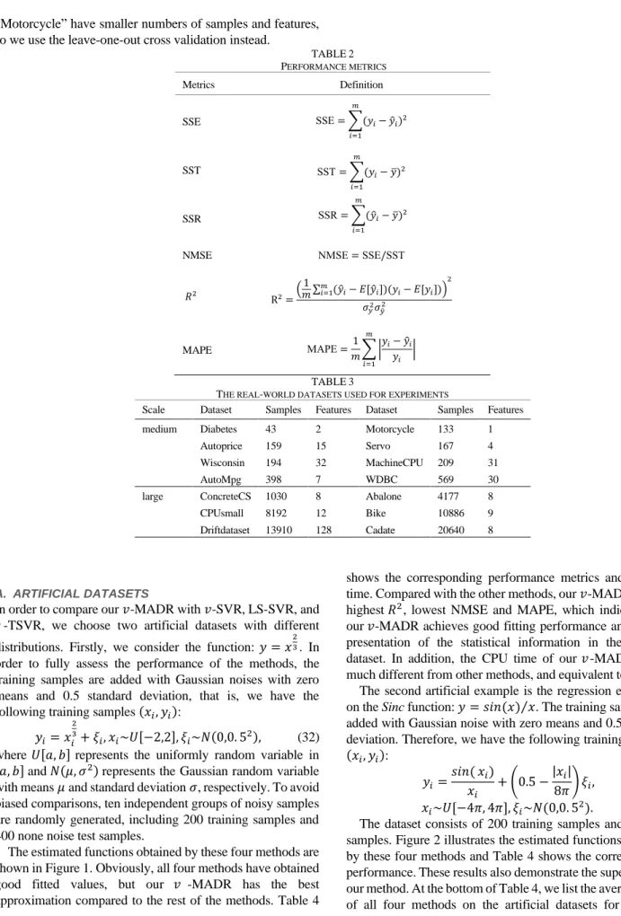
TABLE2 PERFORMANCE METRICS Metrics Definition SSE SSE= ∑(𝑦𝑖− 𝑦̂𝑖)2 𝑚 𝑖=1 SST SSR SST= ∑(𝑦𝑖− 𝑦̅)2 𝑚 𝑖=1 SSR= ∑(𝑦̂𝑖− 𝑦̅)2 𝑚 𝑖=1
NMSE NMSE=SSE/SST
𝑅2 R2=( 1 𝑚∑𝑚𝑖=1(𝑦̂𝑖− 𝐸[𝑦̂𝑖])(𝑦𝑖− 𝐸[𝑦𝑖])) 2 𝜎𝑦2𝜎𝑦̂2 MAPE MAPE=1 𝑚∑ | 𝑦𝑖− 𝑦̂𝑖 𝑦𝑖 | 𝑚 𝑖=1 TABLE3
THE REAL-WORLD DATASETS USED FOR EXPERIMENTS
Scale Dataset Samples Features Dataset Samples Features medium Diabetes 43 2 Motorcycle 133 1
Autoprice 159 15 Servo 167 4 Wisconsin 194 32 MachineCPU 209 31
AutoMpg 398 7 WDBC 569 30
large ConcreteCS 1030 8 Abalone 4177 8 CPUsmall 8192 12 Bike 10886 9 Driftdataset 13910 128 Cadate 20640 8
A. ARTIFICIAL DATASETS
In order to compare our 𝑣-MADR with 𝑣-SVR, LS-SVR, and 𝜀-TSVR, we choose two artificial datasets with different distributions. Firstly, we consider the function: 𝑦 = 𝑥23. In order to fully assess the performance of the methods, the training samples are added with Gaussian noises with zero means and 0.5 standard deviation, that is, we have the following training samples (𝑥𝑖, 𝑦𝑖):
𝑦𝑖= 𝑥𝑖
2 3+ 𝜉
𝑖, 𝑥𝑖~𝑈[−2,2], 𝜉𝑖~𝑁(0,0. 52), (32)
where 𝑈[𝑎, 𝑏] represents the uniformly random variable in [𝑎, 𝑏] and 𝑁(𝜇, 𝜎2) represents the Gaussian random variable
with means 𝜇 and standard deviation 𝜎, respectively. To avoid biased comparisons, ten independent groups of noisy samples are randomly generated, including 200 training samples and 400 none noise test samples.
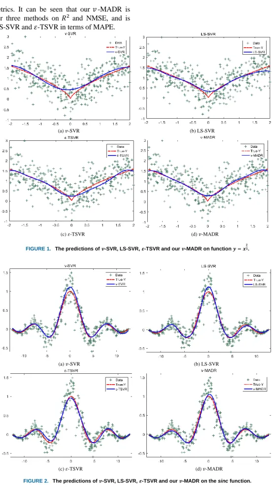
The estimated functions obtained by these four methods are shown in Figure 1. Obviously, all four methods have obtained good fitted values, but our 𝑣 -MADR has the best approximation compared to the rest of the methods. Table 4
shows the corresponding performance metrics and training time. Compared with the other methods, our 𝑣-MADR has the highest 𝑅2, lowest NMSE and MAPE, which indicates that
our 𝑣-MADR achieves good fitting performance and a good presentation of the statistical information in the training dataset. In addition, the CPU time of our 𝑣-MADR is not much different from other methods, and equivalent to 𝑣-SVR. The second artificial example is the regression estimation on the Sinc function: 𝑦 = 𝑠𝑖𝑛(𝑥) 𝑥⁄ . The training samples are added with Gaussian noise with zero means and 0.5 standard deviation. Therefore, we have the following training samples (𝑥𝑖, 𝑦𝑖): 𝑦𝑖= 𝑠𝑖𝑛( 𝑥𝑖) 𝑥𝑖 + (0.5 −|𝑥𝑖| 8𝜋) 𝜉𝑖, 𝑥𝑖~𝑈[−4𝜋, 4𝜋], 𝜉𝑖~𝑁(0,0. 52). (33)
The dataset consists of 200 training samples and 400 test samples. Figure 2 illustrates the estimated functions obtained by these four methods and Table 4 shows the corresponding performance. These results also demonstrate the superiority of our method. At the bottom of Table 4, we list the average ranks of all four methods on the artificial datasets for different
performance metrics. It can be seen that our 𝑣-MADR is superior to other three methods on 𝑅2 and NMSE, and is
comparable to LS-SVR and 𝜀-TSVR in terms of MAPE.
(a) 𝑣-SVR (b) LS-SVR
(c) 𝜀-TSVR (d) 𝑣-MADR
FIGURE 1. The predictions of 𝒗-SVR, LS-SVR, 𝜺-TSVR and our 𝒗-MADR on function 𝒚 = 𝒙𝟐𝟑.
(a) 𝑣-SVR (b) LS-SVR
(c) 𝜀-TSVR (d) 𝑣-MADR
12
TABLE4THE RESULT COMPARISONS OF 𝒗-SVR,LS-SVR,𝜺-TSVR AND OUR 𝒗-MADR ON ARTIFICIAL DATASETS. Dataset regressor 𝑅2 (rank) NMSE (rank) MAPE (rank) CPU(sec) 𝑥23 𝑣-SVR 0.9319(4) 0.0856(4) 0.2479(4) 0.0333 LS-SVR 0.9446(3) 0.0698(3) 0.2152(2) 0.0188 𝜀-TSVR 0.9500(2) 0.0593(2) 0.2091(1) 0.0196 𝒗-MADR 0.9584(1) 0.0529(1) 0.2165(3) 0.0471 𝑆𝑖𝑛𝑐(𝑥) 𝑣-SVR 0.9889(2) 0.0183(2) 1.1792(4) 0.0837 LS-SVR 0.9844(3) 0.0190(3) 0.8389(2) 0.0172 𝜀-TSVR 0.9823(4) 0.0200(4) 0.9118(3) 0.0202 𝒗-MADR 0.9940(1) 0.0083(1) 0.7333(1) 0.0474 average rank 𝑣-SVR 3 3 4 - LS-SVR 3 3 2 - 𝜀-TSVR 3 3 2 - 𝒗-MADR 1 1 2 - B. MEDIUM-SCALE DATASETS
Table 5 and Table 6 list the experimental results on the eight medium-scale datasets from UCI and StatLib with RBF and polynomial kernels, respectively. From the average rank at the bottom of Table 5 and Table 6, our 𝑣-MADR is superior to the other three methods. In detail, on most datasets, our 𝑣-MADR has the highest 𝑅2, lowest NMSE and MAPE. Although on
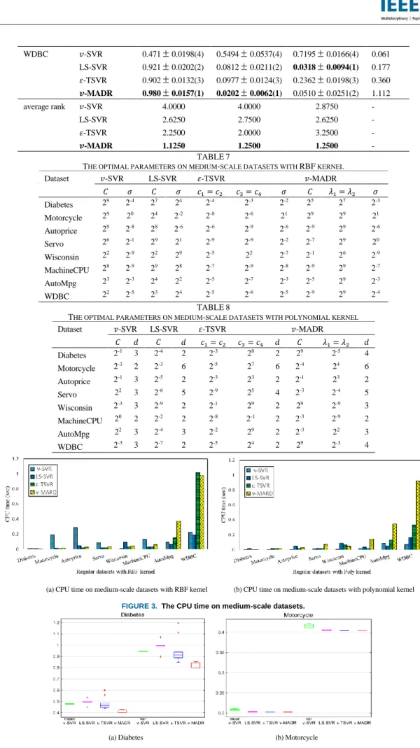
several datasets, such as “MachineCPU”, our 𝑣-MADR does not achieve the best experimental results compared with other methods, it is not the worst. Our 𝑣-MADR also has good performance in terms of CPU running time. The above experimental results indicate that 𝑣-MADR is an efficient and promising algorithm for regression. Table 7 and Table 8 list the optimal parameters with RBF and polynomial kernels, respectively. Figure 3(a) and Figure 3(b) show the comparisons of CPU time among our 𝑣-MADR, 𝑣-SVR, LS-SVR and 𝜀-TSVR on each medium-scale dataset with RBF kernel and polynomial kernel.
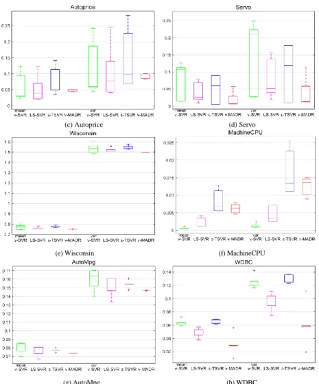
For further evaluation, we investigate the absolute regression deviation mean and variance of our 𝑣-MADR with RBF kernel, 𝑣-SVR, LS-SVR and 𝜀-TSVR on medium-scale datasets as shown in Figure 4. From Figure 4, our 𝑣-MADR has the smallest absolute regression deviation mean and
variance on most datasets. In addition, 𝑣-MADR also has the most compact mean and variance distribution, which demonstrates its robustness. From the above results, it is obvious that our 𝑣-MADR outperforms other three methods.
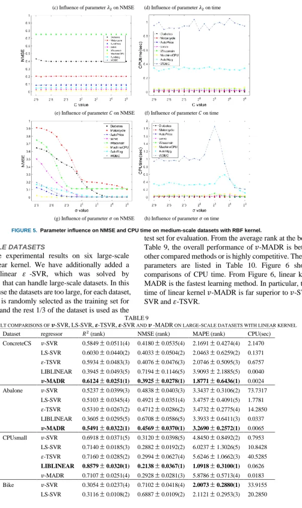
The change of parameter values may have a great effect on the results of regression analysis. For our RBF kernel 𝑣 -MADR, there are mainly three trade-off parameters, i.e., 𝜆1,
𝜆2, 𝐶 and one kernel parameter 𝜎. Figure 5(a) and Figure 5(b)
shows the influence of 𝜆1 on NMSE and CPU time by varying
it from 2−9 to 29 while fixing 𝜆
2, 𝐶 and 𝜎 as the optimal ones
by cross validation. Figures 5(c)~5(h) show the influence of 𝜆2, 𝐶 and 𝜎 on NMSE and CPU time, respectively. As one
can see from Figure 5(a), Figure 5(c) and Figure 5(e), the NMSE values on medium-scale datasets do not change significantly when the values of the three parameters 𝜆1, 𝜆2,
and 𝐶 are changed. Figure 5(g) shows that 𝜎 has more obvious influence on NMSE. On most datasets, as 𝜎 becomes larger, NMSE will become smaller and smaller until it converges at a fixed value. Figure 5(b), Figure 5(d), Figure 5(f) and Figure 5(h) show the influence of parameters 𝜆1, 𝜆2, 𝐶 and 𝜎 on CPU
time. Experimental results indicate that the performance of 𝑣 -MADR is not sensitive to parameter changes, which further demonstrates the robustness of 𝑣-MADR.
TABLE5
THE RESULT COMPARISONS OF 𝒗-SVR,LS-SVR,𝜺-TSVR AND 𝒗-MADR ON MEDIUM-SCALE DATASETS WITH RBF KERNEL
Dataset regressor 𝑅2 (rank) NMSE (rank) MAPE (rank) CPU(sec) Diabetes 𝑣-SVR 0.53430.0028(2) 0.47680.0024(2) 1.59710.0197(4) 0.009 LS-SVR 0.51510.0381(4) 0.49860.0504(4) 1.57420.0477(2) 0.014 𝜀-TSVR 0.52810.1182(3) 0.48050.1185(3) 1.59090.1188(3) 0.004 𝒗-MADR 0.58910.0137(1) 0.41270.0141(1) 1.47500.0493(1) 0.002 Motorcycle 𝑣-SVR 0.79380.0020(3) 0.20810.0029(4) 1.26360.0352(4) 0.007 LS-SVR 0.79750.0011(2) 0.20270.0009(3) 1.24440.0154(3) 0.013 𝜀-TSVR 0.76800.0003(4) 0.20210.0003(2) 1.24410.0055(2) 0.012 𝒗-MADR 0.79840.0006(1) 0.20170.0007(1) 1.23160.0063(1) 0.016 Autoprice 𝑣-SVR 0.94810.0680(2) 0.05300.0698(2) 0.41870.1070(1) 0.004 LS-SVR 0.94650.0674(3) 0.05410.0682(3) 0.50390.1392(3) 0.049 𝜀-TSVR 0.93380.0744(4) 0.06650.0745(4) 0.53550.1524(4) 0.007 𝒗-MADR 0.95490.0040(1) 0.04670.0035(1) 0.48890.0220(2) 0.027 Servo 𝑣-SVR 0.93370.0565(4) 0.06860.0582(4) 0.24910.0420(2) 0.291 LS-SVR 0.96300.0403(2) 0.03720.0406(2) 0.33740.1835(3) 0.019
𝜀-TSVR 0.95070.0445(3) 0.04950.0446(3) 0.39310.2082(4) 0.016 𝒗-MADR 0.97550.0187(1) 0.02530.0320(1) 0.24730.1280(1) 0.045 Wisconsin 𝑣-SVR 0.24200.0354(3) 0.77120.0371(3) 1.82550.1265(4) 0.008 LS-SVR 0.25460.0146(2) 0.75740.0202(2) 1.56670.0462(1) 0.086 𝜀-TSVR 0.22850.0130(4) 0.77520.0137(4) 1.70280.1055(3) 0.027 𝒗-MADR 0.26410.0016(1) 0.74860.0012(1) 1.58400.0125(2) 0.046 MachineCPU 𝑣-SVR 0.99940.0005(1) 0.00060.0006(1) 0.08880.1165(1) 0.006 LS-SVR 0.99780.0020(2) 0.00220.0020(2) 0.17750.1113(2) 0.027 𝜀-TSVR 0.99210.0048(4) 0.00800.0048(4) 0.35800.1641(4) 0.034 𝒗-MADR 0.99420.0014(3) 0.00630.0017(3) 0.21340.0779(3) 0.047 AutoMpg 𝑣-SVR 0.91960.0108(4) 0.08070.0121(4) 1.01110.2842(2) 0.118 LS-SVR 0.92620.0072(2) 0.07410.0079(2) 1.01960.0977(3) 0.054 𝜀-TSVR 0.92280.0034(3) 0.07730.0035(3) 1.05490.0421(4) 0.105 𝒗-MADR 0.92670.0017(1) 0.07360.0015(1) 1.00800.0182(1) 0.326 WDBC 𝑣-SVR 0.93820.0106(3) 0.06320.0086(3) 0.09880.0041(3) 0.216 LS-SVR 0.95200.0109(2) 0.04890.0113(2) 0.01820.0052(1) 0.196 𝜀-TSVR 0.93440.0066(4) 0.06590.0047(4) 0.17260.0085(4) 0.615 𝒗-MADR 0.97100.0258(1) 0.02980.0198(1) 0.07140.0043(2) 0.913 average rank 𝑣-SVR 2.7500 2.8750 2.6250 - LS-SVR 2.3750 2.5000 2.2500 - 𝜀-TSVR 3.6250 3.3750 3.5000 - 𝒗-MADR 1.2500 1.2500 1.6250 - TABLE6
THE RESULT COMPARISONS OF 𝒗-SVR,LS-SVR,𝜺-TSVR AND 𝒗-MADR ON MEDIUM-SCALE DATASETS WITH POLYNOMIAL KERNEL
Dataset regressor 𝑅2 (rank) NMSE (rank) MAPE (rank) CPU(sec) Diabetes 𝑣-SVR 0.3710.0931(4) 0.64240.1007(4) 1.21350.5799(2) 0.001 LS-SVR 0.5260.0096(2) 0.49010.0313(3) 1.49290.1274(3) 0.012 𝜀-TSVR 0.5250.0063(3) 0.48460.0214(2) 1.67950.1074(4) 0.004 𝒗-MADR 0.5490.0324(1) 0.48340.0317(1) 1.12540.0465(1) 0.002 Motorcycle 𝑣-SVR 0.1150.0106(4) 0.88980.0103(4) 1.27300.1945(1) 0.001 LS-SVR 0.5470.0024(3) 0.45440.0055(3) 1.69290.0356 (4) 0.014 𝜀-TSVR 0.5480.0010(2) 0.45400.0042(2) 1.67710.0540 (3) 0.032 𝒗-MADR 0.5490.0006(1) 0.45160.0028(1) 1.64560.0315 (2) 0.017 Autoprice 𝑣-SVR 0.8810.0433(4) 0.12170.0551(4) 0.65010.1275(4) 0.004 LS-SVR 0.9650.0109(3) 0.03490.0113(3) 0.41840.0446(2) 0.043 𝜀-TSVR 0.9730.0082(2) 0.03150.0152(2) 0.47500.1303(3) 0.017 𝒗-MADR 0.9760.0108(1) 0.02560.0115(1) 0.40560.0772(1) 0.025 Servo 𝑣-SVR 0.5450.0034(4) 0.49050.0079(4) 0.80680.0122(4) 0.016 LS-SVR 0.9350.0385(3) 0.06450.0384(3) 0.48700.1473(3) 0.020 𝜀-TSVR 0.9420.0012(2) 0.05760.0017(1) 0.48560.0112(2) 0.019 𝒗-MADR 0.9450.0047(1) 0.06310.0066(2) 0.44250.1647(1) 0.083 Wisconsin 𝑣-SVR 0.2030.0227(4) 0.83260.0357(4) 1.30110.0160(2) 0.007 LS-SVR 0.4690.0021(3) 0.56920.0092(3) 1.36140.0036(3) 0.095 𝜀-TSVR 0.7770.0020(1) 0.24390.0336(1) 1.37930.1926(4) 0.039 𝒗-MADR 0.5850.0013(2) 0.45770.0066(2) 0.82050.0081(1) 0.041 MachineCPU 𝑣-SVR 0.9330.0175(4) 0.06820.0171(4) 1.35250.2995(4) 0.015 LS-SVR 0.9990.0008(3) 0.00060.0009(3) 0.10680.0696(2) 0.029 𝜀-TSVR 0.9990.0004(2) 0.00050.0005(2) 0.11590.0503(3) 0.021 𝒗-MADR 0.9990.0002(1) 0.00040.0003(1) 0.09160.0251(1) 0.045 AutoMpg 𝑣-SVR 0.8020.0127(4) 0.19970.0136(4) 1.25300.2663(2) 0.080 LS-SVR 0.8950.0307(2) 0.10470.0309(2) 1.26130.2146(3) 0.047 𝜀-TSVR 0.8920.0396(3) 0.10790.0356(3) 1.36680.0156(4) 0.143 𝒗-MADR 0.9220.0131(1) 0.08150.0154(1) 1.12190.2950(1) 0.298
WDBC 𝑣-SVR 0.4710.0198(4) 0.54940.0537(4) 0.71950.0166(4) 0.061 LS-SVR 0.9210.0202(2) 0.08120.0211(2) 0.03180.0094(1) 0.177 𝜀-TSVR 0.9020.0132(3) 0.09770.0124(3) 0.23620.0198(3) 0.360 𝒗-MADR 0.9800.0157(1) 0.02020.0062(1) 0.05100.0251(2) 1.112 average rank 𝑣-SVR 4.0000 4.0000 2.8750 - LS-SVR 2.6250 2.7500 2.6250 - 𝜀-TSVR 2.2500 2.0000 3.2500 - 𝒗-MADR 1.1250 1.2500 1.2500 - TABLE7
THE OPTIMAL PARAMETERS ON MEDIUM-SCALE DATASETS WITH RBF KERNEL
Dataset 𝑣-SVR LS-SVR 𝜀-TSVR 𝑣-MADR 𝐶 𝜎 𝐶 𝜎 𝑐1= 𝑐2 𝑐3= 𝑐4 𝜎 𝐶 𝜆1= 𝜆2 𝜎 Diabetes 29 2-4 27 24 2-4 2-3 2-2 25 27 2-3 Motorcycle 29 20 24 2-2 2-8 2-6 21 29 29 21 Autoprice 29 2-8 28 2-6 2-6 2-9 2-6 2-9 29 2-6 Servo 26 2-1 29 21 2-9 2-9 2-2 2-7 29 20 Wisconsin 22 2-9 22 29 2-5 22 2-7 2-1 26 2-9 MachineCPU 28 2-9 29 28 2-7 2-9 2-8 2-9 29 2-7 AutoMpg 23 2-3 24 22 2-5 2-7 2-3 2-5 29 2-3 WDBC 22 2-5 23 24 2-5 2-6 2-5 2-9 29 2-4 TABLE8
THE OPTIMAL PARAMETERS ON MEDIUM-SCALE DATASETS WITH POLYNOMIAL KERNEL
Dataset 𝑣-SVR LS-SVR 𝜀-TSVR 𝑣-MADR 𝐶 𝑑 𝐶 𝑑 𝑐1= 𝑐2 𝑐3= 𝑐4 𝑑 𝐶 𝜆1= 𝜆2 𝑑 Diabetes 2-1 3 2-4 2 2-3 28 2 29 2-5 4 Motorcycle 2-3 2 2-3 6 2-5 27 6 2-4 24 6 Autoprice 2-1 3 2-5 2 2-3 23 2 2-1 23 2 Servo 22 3 2-6 5 2-9 25 4 2-3 2-4 5 Wisconsin 2-3 3 2-9 2 2-1 29 2 29 2-9 3 MachineCPU 20 2 2-2 2 2-8 2-1 2 2-3 2-9 2 AutoMpg 22 3 2-4 3 2-2 29 2 2-3 22 3 WDBC 2-3 3 2-7 2 2-5 24 2 29 2-3 4
(a) CPU time on medium-scale datasets with RBF kernel (b) CPU time on medium-scale datasets with polynomial kernel FIGURE 3. The CPU time on medium-scale datasets.
(c) Autoprice (d) Servo
(e) Wisconsin (f) MachineCPU
(g) AutoMpg (h) WDBC
FIGURE 4. The absolute regression deviation mean and variance of 𝒗-MADR with RBF kernel on medium-scale datasets.