41
SCALAR MIXING AND DISSIPATION RATE IN LARGE-EDDY SIMULATIONS
OF NON-PREMIXED TURBULENT COMBUSTION
HEINZ PITSCHandHELFRIED STEINER Center for Turbulence Research Flow Physics and Computation Division
Stanford University Stanford, CA 94305-3030, USA
Predictions of scalar mixing and the scalar dissipation rate from large-eddy simulations of a piloted non-premixed methane/air diffusion flame (Sandia flame D) using the Lagrangian-type flamelet model are presented. The results obtained for the unconditionally filtered scalar dissipation rate are qualitatively compared with general observations of scalar mixing from experiments in non-reactive and reactive jets. In agreement with experimental data, provided the reaction zone has an inward direction, regions of high scalar dissipation rate are organized in layerlike structures, inwardly inclined to the mean flow and aligned with the instantaneous reaction zone. The analysis of single-point time records of the mixture fraction reveals ramplike structures, which have also been observed experimentally and are believed to indicate large-scale turbulent structures. The probability density function (pdf) of the instantaneous resolved scalar dissipation rate at stoichiometric mixture evaluated at cross sections normal to the the nozzle axis is shown to be described accurately by a lognormal pdf withr⳱1. A new model for the conditionally averaged scalar dissipation rate has been proposed and is shown to account for local deviations from the simple mixing layer structure. The stabilizing effect of the pilot flame in the present configuration is also discussed. Finally, the influence of the resolved fluctuations of the scalar dissipation rate on the flame structure is investigated, revealing only a weak influence on temperature and nitric oxide predictions. However, the model requires further refinement for situations in which local extinction events become important.
Introduction
The mixing of scalars in turbulent flows is a very interesting problem which provides a fundamental understanding of the basic processes involved in non-premixed combustion problems and has been investigated by many in this field. A comprehensive review of experimental findings has recently been provided by Pitts et al. [1].
In non-premixed combustion, chemical reactions occur only if fuel and oxidizer are mixed at the molecular level. Although turbulent mixing is re-sponsible for stirring the reactants at large scales, it contributes to the molecular scalar mixing only in-directly, increasing the scalar variances and thereby the scalar gradients. Molecular mixing essentially oc-curs at the smallest turbulent scales by removal of the scalar variance. The rate of molecular scalar mix-ing is represented by the scalar dissipation rate, which can be identified as the most important pa-rameter in the description of non-premixed com-bustion.
Because combustion can occur only if the reac-tants are mixed on the molecular level, the scalar dissipation rate provides a measure of the maximum possible chemical reaction rate. This is the basic idea of the eddy break-up model [2]. Assuming infinitely
fast chemistry, it has been shown by Bilger [3] that the turbulent reaction rate is linearly proportional to the scalar dissipation rate at stoichiometric condi-tions,vst. For finite-rate chemistry, the scalar
dissi-pation rate appears as a parameter in most of the commonly applied combustion models such as the flamelet model [4,5], the transported probability density function model [6,7], and the conditional moment closure model [8].
The influence of the scalar dissipation rate,v, on the structure of diffusion flames has been discussed by Peters [4]. In general, the scalar dissipation rate at the stoichiometric mixture fraction describes the departure from chemical equilibrium. If the stoi-chiometric scalar dissipation rate in a steady laminar diffusion flame exceeds a critical value,vq, the flame
will be quenched. However, it has been found in experiments [9,10] and numerical simulations [11– 13] that the flame structure cannot instantaneously follow changes invstand that in the case of a
fluc-tuating scalar dissipation rate, instantaneous values ofvstcan by far exceed vqwithout quenching the
flame. On the other hand, it is possible for the mean scalar dissipation rate to be smaller thanvqand yet
the flame may be quenched by fluctuations above this limit. In situations where local quenching oc-curs, it might therefore be of great importance to
accurately model the fluctuations of the scalar dis-sipation rate.
For the modeling of the scalar dissipation rate, large-eddy simulations have the advantage of resolv-ing the major part of the turbulent motion. Only the fluctuations which occur on smaller length scales than the filter width, typically given by the spacing of the numerical discretization, have to be modeled. The modeling effort of the basic quantities such as subgrid scale stresses and variances is supported by the concept of a turbulent energy cascade in two different ways. First, most of the turbulent energy is in the resolved scales. Second, the energy cascade concept suggests that subgrid quantities can be uni-versally related to the resolved field. In contrast, since the dissipation of scalar variance occurs essen-tially at the smallest scales, the major part of the scalar dissipation rate has to be modeled. Following the energy cascade concept, the scalar dissipation rate is, similar to the turbulent kinetic energy dissi-pation rate, a universal quantity describing the scalar variance transport in wavenumber space, and knowl-edge of the resolved-scale field should hence be ben-eficial in the determination of the scalar dissipation rate as a fluctuating quantity.
In this paper, we describe and evaluate the mod-eling of the scalar dissipation rate and its fluctuations in large-eddy simulations (LES) for non-premixed combustion using the Lagrangian-type flamelet model [14,15]. The predictions of the unconditional mean scalar dissipation rate from an LES of a piloted turbulent diffusion flame (Sandia flame D [16,17]) is discussed and compared to general and mainly qualitative observations from several experiments. The influence of resolved fluctuations of the mod-eled conditional scalar dissipation rate on the chem-ical flame structure is investigated by comparing the results of calculations, which include the fluctuations of the scalar dissipation rate, with results for the same configuration obtained by using time-averaged values for the scalar dissipation [18].
We first give a brief review of the Lagrangian-type flamelet model as a combustion model for LES and present a new model for the evaluation of the con-ditional mean scalar dissipation rate. We then discuss the results for the unconditional resolved scalar dis-sipation rate, and finally the influence of the resolved fluctuations of the conditional mean scalar dissipa-tion rate.
Model Formulation Large-Eddy Simulation
The system of equations to be solved is given by the spatially filtered continuity, momentum, and mixture fraction equations provided, for instance, by
Moin et al. [19]. The subgrid stresses and the veloc-ity-mixture fraction covariance appearing in the mo-mentum equations and in the mixture fraction equa-tion are expressed by eddy-viscosity-type models, where the eddy viscosity is given by the Smagorinsky model, the eddy diffusivity, Dt, by the assumption of
a constant turbulent Schmidt number, Sct ⳱ 0.4
[18]. Following Pierce and Moin [19], the mixture fraction variance is given by
2 2 ˜ 2
˜
Z⬙ ⳱CZD (ⵜZ) (1)
The Smagorinsky coefficient and the coefficient CZ
are computed from the solution of the resolved scales by applying the dynamic procedure [20]. No model constants have to be specified in the com-putation of the flow field. The simulation was per-formed in a spherical coordinate system with 192 cells in the downstream direction, 110 cells in the cross-flow direction, and 48 cells in the azimuthal direction. The inflow conditions were prescribed ac-cording to the experimental conditions. Detailed in-formation on the numerical procedure has been given in Ref. [18].
Lagrangian-Type Flamelet Model
In the present simulations, the Lagrangian-type flamelet model was employed to describe turbu-lence/chemistry interactions. The model was devel-oped in the framework of Reynolds averaged simu-lations [14,15] and was recently applied in LES [18]. The model follows the conserved scalar approach, implying that the temperature and the species mass fraction can be related to the mixture fraction. Thus, density-weighted filtered quantities are given by
1
˜ ˜
⳱
冮
(Z)P(Z)dZ (2)0
wherestands for the temperature, T, and the spe-cies mass fractions, Yi. P˜(Z) is the subgrid scale Favre
probability density function (pdf) of the mixture fraction, Z, which is presumed to be ab-function, whose shape is determined by the resolved mixture fraction and its subgrid scale variance. The function Yiis given by the solution of the unsteady flamelet
equations. For the species mass fractions, for ex-ample, these are given as
2
Yiⳮq vYiⳮ m˙ ⳱ 0 (3) i
2 s 2 Z
Here,sis the Lagrangian flamelet time,qis the den-sity, m˙iis the chemical production rate per unit
vol-ume, and following Ref. [14],vis given by the con-ditional scalar dissipation rate 具v|Z典 (s). Lewis numbers of the chemical species have been assumed to be unity. Lagrangian flamelet particles are as-sumed to be introduced at the nozzle exit and travel downstream essentially with the axial velocity at stoi-chiometric mixture fraction. Then,scan be related
to the physical space coordinate in the axial direction x as x 1 s ⳱
冮
dx⬘ (4) ˜ 0 具u˜ |Z˜Z st典(x⬘, t)where具u˜Z˜|Z˜st典denotes the velocity of the
stoichio-metric mixture fraction surface in the axial direction. The resolved mass fractions can then be determined as a function of time and space with equations 2, 3, and 4, provided the conditional scalar dissipation rate is given as a function of the flamelet time,s, and the mixture fraction, Z.
Scalar Dissipation Rate
The unconditionally filtered scalar dissipation rate is expressed in terms of the eddy diffusivity and the gradient of the resolved mixture fraction using the first-order model given by Girimaji and Zhou [21] as
2
˜
v˜ ⳱ 2(DZⳭ D ) (t ⵜZ) (5)
where DZis the molecular diffusivity of the mixture
fraction.
As pointed out earlier, the temporal development of the scalar dissipation rate appearing in equation 3 is unknown and has to be related to the uncondi-tional mean given by equation 5. A common ap-proach to achieve this is to presume the functional dependence of the scalar dissipation rate on the mix-ture fraction as具v|Z典⳱具vst典f(Z), using analytic
ex-pressions for the function f(Z) as suggested in the literature [4,14,22]. Then, it is sufficient to deter-mine the value conditioned on stoichiometric mix-ture.具vst典can then be determined by introducing the
expression for具v|Z典in the equation for the filtered scalar dissipation rate,v˜,which can be written as
1
˜
v˜ (x, t) ⳱
冮
具v|Z典 (x, t)P(Z, x, t)dZ (6)Z⳱0
It is demonstrated below that the function f(Z) cannot be represented by the commonly applied ex-pressions for unsteady mixing layers or counterflow diffusion flames, since in the present study a piloted flame is considered.
Here, a new model for the computation of the conditional average of the scalar dissipation rate, which has to be specified as a function of the axial distance from the nozzle as具v|Z典(x, t), is proposed. This model is similar to the approach used by Bushe and Steiner [23] for the estimation of chemical source terms. The term具v|Z典(x, t) is computed by the inversion of the integral in equation 6. Writing equation 6 for each computational cell in a chosen plane normal to the nozzle axis gives
1
˜
v˜ (x, t)i ⳱
冮
具v|Z典 (x, t)P (Z, x, t)dZ,i Z⳱0i ⳱1, . . . , N (x)c (7)
Here, Nc(x) is the number of cells in the plane
con-sidered. If the continuous function具v|Z典(Z, x, t) in
equation 7 is approximated by a discrete represen-tation in terms of the mixture fraction as具v|Zj典(x, t),
j ⳱ 1, . . . , NZ, where NZdenotes the number of
values used to represent the mixture fraction space, the integral in equation 7 can be approximated by a sum using, for example, the trapezoidal integration rule as
NZ
v˜ (x, t)i ⬇
兺
Aij具v|Z典 (Z , x, t),j j⳱1j ⳱ 1, . . . , NZ (8)
where the coefficient matrix Aijcontains the
discre-tized pdf P˜i(Zj, x, t) and the coefficients of the
nu-merical integration scheme.
Equation 8 represents a system of Nc(x) equations
for NZunknowns. For Nc(x)⬎NZ, this can be solved
by minimizing the resulting error of the overdeter-mined system via a least squares approach.
An alternative method to compute the conditional scalar dissipation rate has been proposed by Janicka and Peters [24]. In the transport equation of the mix-ture fraction pdf [7], the conditional scalar dissipa-tion rate appears in the term representing molecular mixing. If the mixture fraction pdf is prescribed, this equation can be used to determine具v|Z典. The un-derlying assumptions of this approach, which in-clude the use of modeled values of the unconditional mean and assumedb-function shape of the mixture fraction pdf, are very similar to the model presented here. In contrast to this, the pdf transport equation method in principle provides averages over one computational cell, while the method proposed in this work is an average over a larger number of cells. However, for small values of the mixture fraction pdf, the determination of the conditional scalar dis-sipation rate from the pdf transport equation be-comes singular, which makes its application difficult, particularly in LES, where the subgrid pdf is non-zero only in a very narrow range around the mean.
Results and Discussion
In this section, the predicted results for scalar mix-ing and the scalar dissipation rate from an LES of a piloted non-premixed methane/air diffusion flame (Sandia flame D) with a Reynolds number of Re⳱ 22000 are presented and discussed. The instanta-neous conditional scalar dissipation rates, which are obtained in the LES from equation 8, have been averaged in time and then used in the solution of the flamelet equations. This assumption is discussed below.
Experimental data for axial velocity and root mean square (RMS) has been determined by Hassel [25], while data for the mean and RMS of the tempera-ture, and mean and conditional mean mass fractions of the chemical species CH4, O2, H2, H2O, CO,
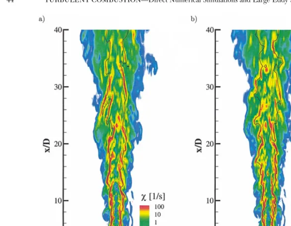
Fig. 1. Resolved instantaneous scalar dissipation rate distribution. Results in (b) are at a time 20 ms later than those in (a).
CO2, OH, and NO have been given by Barlow et al.
[16,17]. Comparison of the predicted results with the experimental data has been presented and dis-cussed further in Ref. [18]. In general, the agree-ment of predictions and experiagree-mental data is consid-ered very good.
Unconditionally Filtered Scalar Dissipation Rate Spatial -distributionv˜
Figure 1 shows instantaneous distributions of the unconditionally filtered scalar dissipation rate,v˜, ob-tained from equation 5. Figure 1b shows a realiza-tion at a time approximately 20 ms later than that in 1a. The figures are presented at the same point in time as the temperature distributions given in Ref. [18]. The stoichiometric contour, which indicates the approximate location of the reaction zone, is also in-dicated. Regions of high scalar dissipation rate ap-pear in layerlike structures, which are directed in-ward. In general, these layers are well aligned with the stoichiometric contour, when this is directed in-ward. Since both the stoichiometric contour and the
high scalar dissipation rate layers cannot be inclined to the mean flow over a long distance, the stoichio-metric contour diverges outward again to the next surrounding dissipation layer. This usually occurs at much higher angles relative to the axis of the jet. Since the inwardly directed stoichiometric contours appear at high scalar dissipation rate, the corre-sponding temperature distribution is very narrow, as corroborated by Ref. [18]. In contrast, the outwardly directed contours are associated with broad tem-perature regions.
Similar behavior has been observed by Feikema et al. [26] in measurements of the scalar dissipation rate in a non-reacting turbulent jet. They found that the scalar dissipation rate appears in layers, which are inclined at approximately 45⬚to the flow. Rehm and Clemens [27,28] found that the minimum com-pressive strain in turbulent jet flames appears in similar layers, which are also inclined at 45⬚to the flow and aligned with the reaction zone. Rehm and Clemens [28] have also shown from experiments in non-reacting jets that the minimum compressive strain layers are well aligned with the scalar dissi-pation rate layers. In experiments of reactive jets,
Fig. 2. Time records of the resolved mixture fraction and the scalar dissipation rate on the centerline at x/D⳱ 30.
Fig. 3. The pdf of the stoichiometric resolved scalar dis-sipation rate at x/D⳱15 and x/D⳱30 (solid lines) com-pared to log-normal pdfs (dashed lines), withr⳱1 from equation 9.
they also observed the broadening of the reaction zone in instances where this is directed away from the jet axis. All these findings are consistent with the current simulation. However, on average the incli-nation angle of the dissipation layers in Fig. 1 seems to be smaller than 45⬚to the direction of the flow. Single-point time records of Z˜ and ˜v
Single-point time records of the mixture fraction and the scalar dissipation rate at the centerline po-sition at x/D⳱30 are given in Fig. 2. As shown in Fig. 2 and also by Pitts et al. [1] for non-reacting jet experiments, the scalar dissipation rate fluctuates at a much higher frequency than the mixture fraction. Also, the mean duration of a peak at high scalar dis-sipation rate appears to be much longer than a peak at low scalar dissipation rate. Donbar et al. [10] found that for a turbulent jet flame with a Reynolds number Re⳱18,600, which is very similar to the present case, that the strain rate fluctuates at ap-proximately 10 kHz. The frequency of the scalar dis-sipation rate fluctuations at x/D⳱30 shown in Fig. 2 can be estimated to be 2.5 kHz. This frequency however, varies strongly with the nozzle distance.
It should be noted here that even the shortest fluc-tuations appearing in Fig. 2 are well resolved in time, such that the time-step of the calculation does not impose any filtering. The frequency that can be re-solved by the computational mesh might be esti-mated by the average cell size in the axial direction and the time averaged axial velocity as fRes⬇10 kHz.
Since it has been found in the reacting jet experi-ments of Donbar et al. [10] and also in simulations of counterflow diffusion flames by Saitoh and Otsuka [9] that the flame chemistry does not respond to fluc-tuations in the strain rate higher than 10 kHz, it ap-pears that the spatial filtering is not restrictive for the use of the predicted scalar dissipation rate in chemistry calculations.
Figure 2 also reveals one other very important mixing aspect which is not directly related to the
scalar dissipation, but should still be discussed here. Pitts et al. [1] have investigated large-scale turbulent structures in a non-reacting jet. As one of the most important proofs of the formation of these tures, they discuss the observation of ramplike struc-tures in one-point time records of scalars in turbu-lent jets. These ramplike structures can also be observed in the resolved mixture fraction record shown in Fig. 2. In general, the increase of the mix-ture fraction occurs much more rapidly than the fol-lowing decrease. This seems to corroborate that the current simulations are capable of describing large-scale mixing phenomena, which are believed to be very important for the overall structure and devel-opment of the scalar field.
The pdf of ˜v
The pdf of the scalar dissipation rate has been in-vestigated in many studies [1,29,30]. It has been found that the distribution ofv is log-normal. In terms of the density-weighted filtered quantities, this can be expressed as
2
1 (lnv˜ ⳮl)
˜P(v˜ )⳱ exp
冢
ⳮ 2冣
(9)2r v˜ 2冪 p
Here,landrare parameters of the pdf, which es-sentially represent the mean and the fluctuation about the mean, respectively. From non-reacting jet experiments, Effelsberg and Peters [29] have found the parameterrto have a value close to unity. The evaluation of the pdf ofv˜stusing all computational cells in the particular cross-section is presented in Fig. 3 for x/D⳱15 and x/D⳱30. Also shown is the pdf evaluated from equation 9 withr⳱1 and the appropriate values forlto match the mean sca-lar dissipation rate, viz.l⳱4.7 and 3.2 for x/D⳱ 15 and 30, respectively. The comparison shows that
Fig. 4. Conditional scalar dissipation rate at different downstream locations. Also shown is a commonly pre-sumed form of the mixture fraction dependence of the sca-lar dissipation rate.
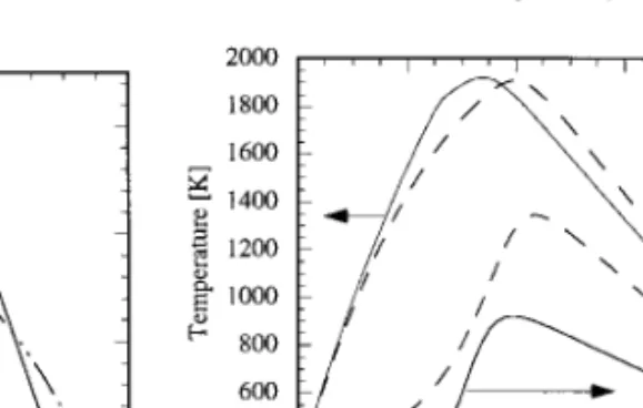
Fig. 5. Influence of the mixture fraction dependence of the scalar dissipation rate on the flamelet solution at the nozzle exit. Calculation usingv(Z) from equation 8 (solid lines) compared to solution withv(Z) (dashed lines) pre-sumed according to Ref. [14].
the distribution ofv˜stat both positions is almost per-fectly log-normal, and also thatr⳱1 seems to be a very good approximation for the case investigated. The same value ofris observed at x/D⳱45.
Conditional Mean Scalar Dissipation Rate
Results for the conditional mean scalar dissipation rate at different downstream locations determined from equation 8 are shown in Fig. 4. The comparison with a presumed shape ofv(Z) from Ref. [14] indi-cates that this simple function is not applicable in the present case. Within the pilot stream, which is at Z⳱0.27, the scalar gradient, and hence the scalar dissipation rate, is zero. Even at far downstream lo-cations, the shape of the scalar dissipation rate is still influenced by the pilot flame.
The computed shape at x/D⳱1 provides an in-teresting explanation of the stabilizing effect of a pi-lot flame. The pipi-lot causes the scalar dissipation rate to be zero at the pilot mixture fraction, which in turn also causes the scalar dissipation rate at stoichio-metric mixture fraction (Zst ⳱ 0.35) to be small.
However, by interdiffusion with the surrounding mixing layer this value strongly increases with down-stream direction. Also, the same diffusive effect causes the scalar dissipation rate generally to de-crease strongly with downstream direction [31]. Hence, in the present case,vstfirst increases until approximately x/D⳱7.5, and then decreases. If the maximum value stays smaller than the extinction limit,vst,q, the flame stabilizes at the pilot. However,
if it exceedsvst,q, the flame will exhibit local
extinc-tion or even blow off. This also explains why it is favorable to have the pilot mixture fraction close to the stoichiometric mixture fraction, which keepsvst
lower, and also to have a broad pilot flow, because
then the increase ofvaround the pilot will be much slower.
The influence of the scalar dissipation rate model on the initial conditions for the unsteady flamelet calculation, which is assumed to be the steady flame-let solution withv(Z) evaluated from equation 8 at x/D⳱ 0, is given in Fig. 5. The flamelet solution for the temperature and the CO mass fraction are compared to the solution using the presumedv(Z) of Ref. [14]. Because of the influence of the pilot, the flame is substantially shifted to the lean side. Also, as shown in Fig. 4, the presumed function overestimates the scalar dissipation in the lean part of the flame, leading to a substantial overprediction of the CO mass fraction.
Influence of Resolved Scalar Dissipation Rate Fluctuations
The influence of the scalar dissipation rate fluc-tuations, which are resolved by equation 8, are in-vestigated next. As mentioned above, the pdf of the unconditional scalar dissipation rate clearly reveals a log-normal shape withr ⳱ 1. Because the condi-tional scalar dissipation rate given by equation 8 is a spatial conditional average, which has for the present study and for the results presented in Ref. [18] been performed over all computational cells in cross sec-tions normal to the jet axis, the pdf of具v|Z典is much narrower than the pdfs shown in Fig. 3. This, how-ever, can be substantially improved by sampling over smaller areas. In order to analyze the influence of the resolved fluctuations on the flame structure, 250 different instantaneous scalar dissipation rate and mixture fraction fields were recorded from the cal-culations presented in Ref. [14]. These calcal-culations were performed using the time-averaged scalar dis-sipation rate. Using these data, 250 unsteady flame-let calculations were performed, and the resolved
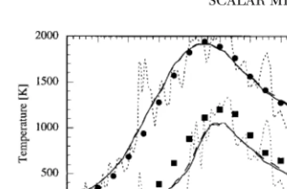
Fig. 6. Ensemble-averaged temperature and NO mass fraction determined as the average over multiple instan-taneous realizations (solid lines) compared to a calculation using a time average of the scalar dissipation rate (dashed lines). Also given is an example for one instantaneous re-alization (dotted line).
temperature and mass fractions were evaluated us-ing equation 2. The results were ensemble averaged, and the temperature and the NO mass fraction of these calculations are compared along the centerline to the calculations using the time average of the sca-lar dissipation rate and the experimental data given by Barlow et al. [16,17] in Fig. 6. Also given in Fig. 6 is one example of an instantaneous solution of tem-perature and NO mass fraction. This solution shows temperature fluctuations, which can be of the order of 700 K. However, almost no differences in the re-sults of both methods can be observed, indicating that the resolved fluctuations of the scalar dissipation rate influence the flame structure only very weakly, and also that the strong fluctuations in the instanta-neous solution given in Fig. 6 are essentially caused by fluctuations in the resolved mixture fraction and its subgrid scale variance. Both methods yield good agreement with the experimental data for the pres-ent case. However, if local extinction evpres-ents start to become important, the pdf of the scalar dissipation rate has to be determined much more accurately, and averages over complete cross sections can no longer be used.
Conclusions
The present study provides a discussion of scalar mixing and the scalar dissipation rate in large-eddy simulations. The results from an LES of the Sandia flame D have been used to compare the predictions of the mixture fraction field and the scalar dissipation rate with mostly qualitative experimental data. In agreement with experimental data, it has been found that regions of high scalar dissipation rate are orga-nized in layerlike structures that are inwardly in-clined to the mean flow and aligned with the reaction zone.
The fluctuation frequency of the scalar dissipation rate has been discussed in the context of the spatial and temporal resolution of the current simulation, and the findings are that the resolution used in the present investigation is not restrictive for the pre-dictions of the scalar dissipation rate. Single-point time records of the mixture fraction have been found to reveal ramplike structures, which are also evident in experimental data for non-reacting jets. Pitts et al. [1] regarded this as one of the most important proofs for the occurrence of large-scale turbulent structures in turbulent jets.
The pdf of the stoichiometric scalar dissipation rate was found to be described accurately by a log-normal pdf with a value ofr⳱1. The ratio of the integral time scales of scalar and velocity fluctua-tions, which is commonly used in Reynolds-averaged turbulence models to determine the unconditionally averaged scalar dissipation rate, was evaluated using the resolved velocity and scalar field.
A model for the conditional scalar dissipation rate has been suggested that accounts for the influence of local deviations from a simple mixing layer struc-ture. Furthermore, this model has been demon-strated to account for the strong influence of a pilot in the near-field of a turbulent jet flame.
Finally, the influence of the fluctuations resolved by the model for the conditional scalar dissipation rate on the flame structure was investigated by com-paring averages over simulations using instantaneous scalar dissipation rate histories with a simulation us-ing the time-averaged scalar dissipation rate. The re-sults for temperature and NO mass fraction are not influenced by the scalar dissipation rate fluctuations. However, the model would need to be refined for instances in which local extinction events become important.
Acknowledgments
Support by the U.S. Department of Energy within the ASCI program is acknowledged. The authors also thank George Kosa´ly for many helpful discussions.
REFERENCES
1. Pitts, W. M., Richards, C. D., and Levenson, M. S., Large- and Small-Scale Structures and Their Interac-tions in an Axisymmetric Jet, NIST internal report NISTIR 6393, National Institute of Standards and Technology, Gaithersburg, MD, 1999.
2. Spalding, D. B., Proc. Combust. Inst. 13:649–657 (1971).
3. Bilger, R. W., Combust. Sci. Technol. 110:155–170 (1976).
4. Peters, N., Prog. Energy Combust. Sci. 10:319–339 (1984).
6. Pope, S. B., Prog. Energy Combust. Sci. 11:119–192 (1985).
7. O’Brien, E. E., in Turbulent Reacting Flows, (P. A. Libby and F. A. Williams, eds.), Springer, 1980, p. 185. 8. Klimenko, A. Y., and Bilger, R. W., Prog. Energy
Com-bust. Sci. 25:595–687 (1999).
9. Saitoh, T., and Otsuka, Y., Combust. Sci. Technol. 12:135–146 (1976).
10. Donbar, J. M., Driscoll, J. F., and Carter, D. C., Com-bust. Flame, in press (2000).
11. Barlow, R. S., and Chen, J.-C., Proc. Combust. Inst. 24:231–237 (1992).
12. Haworth, D. C., Drake, M. C., Pope, S. B., and Blint, R. J., Proc. Combust. Inst. 24:589–597 (1988). 13. Mauss, F., Keller, D., and Peters, N., Proc. Combust.
Inst. 25:693–698 (1990).
14. Pitsch, H., Chen, M., and Peters, N., Proc. Combust. Inst. 27:1057–1064 (1998).
15. Pitsch, H., Combust. Flame, in press, (1999). 16. Barlow, R. S., and Frank, J. H., Proc. Combust. Inst.
27:1087–1095 (1998).
17. www.ca.sandia.gov/tdf/Workshop.html, Sandia Na-tional Laboratory, 1998 (updated June 7, 2000). 18. Pitsch, H., and Steiner, H., unpublished work (1999). 19. Pierce, C. D., and Moin, P., Phys. Fluids A 10:3041–
3044 (1998).
20. Moin, P., Squires, K., Cabot, W., and Lee, S., Phys. Fluids A 3:2746–2757 (1991).
21. Girimaji, S. S., and Zhou, Y., Phys. Fluids A 8:1224– 1236 (1996).
22. Kim, J. S., and Williams, F. A., SIAM J. Appl. Math. 53:1551–1566 (1993).
23. Bushe, W. K., and Steiner, H., Phys. Fluids A 11:1896– 1906 (1999).
24. Janicka, J., and Peters, N., Proc. Combust. Inst. 19:367–374 (1982).
25. Hassel, E., www.ca.sandia.gov/tdf/Workshop.html, Sandia National Laboratory, 1998 (updated June 7, 2000).
26. Feikema, D. A., Everest, D., and Driscoll, J. F., AIAA J. 34:2531–2538 (1996).
27. Rehm, J. E., and Clemens, N. T., Proc. Combust. Inst. 27:1113–1120 (1998).
28. Rehm, J. E., and Clemens, N. T., “The Association of Scalar Dissipation Rate Layers and OH Zones with Strain, Vorticity, and 2-D Dilatation Fields in Turbu-lent Nonpremixed Jets and Jet Flames,” AIAA paper 99-0676, Thirty-Seventh AIAA Aerospace Sciences Meeting and Exhibit, Reno, NV, Jan. 11–14, 1999. 29. Effelsberg, E., and Peters, N., Proc. Combust. Inst.
22:693–700 (1988).
30. Dahm, W. J. A., and Buch, K. A., Phys. Fluids A 1:1290–1293 (1989).
31. Peters, N., and Williams, F. A., AIAA J. 21:423–429 (1983).
COMMENTS
William Mell, University of Utah, USA.1. Did you also implement a quasi-steady version of the flamelet model? If so, how did it perform compared to your transient model?
2. What boundary conditions did you use for the laminar flamelet model? In particular, were transient effects important?
3. Did you consider regimes in which buoyancy played a greater role (rather than momentum) in the flow? It seems likely that in such a situation the axial velocity (which gives the Lagrangian time) may not be as rep-resentative of the flamelets at a given axial position. Author’s Reply.
1. Predictions using a quasi-steady model have been shown to be more accurate if radiation is neglected. For the investigated configuration, the application of the quasi-steady model leads thereby to an iction of the temperature. This leads to an overpred-iction of the NO mass fraction by approximately a fac-tor of 2. However, for the conclusions of the present paper regarding the scalar mixing process, the use of a quasi-steady model will show hardly any influence. 2. Using the models proposed in the present paper, the
predicted conditional scalar dissipation rate becomes small if the pdf of the mixture fraction goes to zero.
This can be seen in Fig. 4. In the region of zero scalar dissipation rates, the diffusion term in the flamelet equation is zero. This implies that the boundary con-ditions of the flamelet solution are homogeneous re-actor solutions at an effective maximum mixture frac-tion.
3. We did not consider a configuration where buoyancy is important. However, the Lagrangian time can still be determined from the axial velocity, which would change accordingly if the momentum flux were domi-nated by buoyancy.
●
A. Y. Klimeuto, The University of Queensland, Austra-lia. I am certain that the topic of the presentation, inves-tigation into the influence of fluctuations of the conserved scalar-dissipation on combustion, is most important for flamelet modeling. However, I think that one question needs some clarification. The subgrid model used by the authors ignores the subgrid fluctuations which can be ex-pected to be most significant for the scalar dissipation. Can this factor affect the conclusions of the present work? Author’s Reply. In the present model, the subgrid part of the scalar dissipation rate is considered by the use of a subgrid model. Because of the subgrid filtering, the pdf
of the scalar dissipation rate and also the frequency of its fluctuations might be influenced. It is shown in Fig. 3 that the resolved pdf is in good agreement with experimental findings. This suggests that the filtering only influences the tails of the pdf. It is also mentioned in the paper that the present simulation can resolve a frequency of 10 kHz. It has been shown in experiments (Ref. [10] in this paper) and simulations of counterflow diffusion flames (Ref. [9] in this paper) that the flame chemistry does not respond to higher frequencies.
●
Andrew Pollard, Queen’s University, Canada. Can you confirm that the scalar dissipation is coincident with regions of high axial vorticity (i.e., braids between azi-muthal vortex rings)?
Author’s Reply. Obviously, the regions of high scalar dissipation rate are located between large-scale azimuthal vortical structures. However, from the observations we made in this study there is not clear evidence that these structures appear in rings, which would be connected by secondary axial vortices. This might still be the case, but we have not looked explicitly into these details.