Nonparametric Predictive Regression

(1)

Singapore Management University

Institutional Knowledge at Singapore Management University

Research Collection School Of Economics

School of Economics

4-2015

Nonparametric Predictive Regression

Ioannis KASPARIS

University of Cyprus

Elena ANDREOU

University of Cyprus

Peter C. B. PHILLIPS

Singapore Management University

, [email protected]

DOI:

https://doi.org/10.1016/j.jeconom.2014.05.015

Follow this and additional works at:

https://ink.library.smu.edu.sg/soe_research

Part of the

Econometrics Commons

This Journal Article is brought to you for free and open access by the School of Economics at Institutional Knowledge at Singapore Management University. It has been accepted for inclusion in Research Collection School Of Economics by an authorized administrator of Institutional Knowledge at Singapore Management University. For more information, please [email protected].

Citation

KASPARIS, Ioannis; ANDREOU, Elena; and PHILLIPS, Peter C. B.. Nonparametric Predictive Regression. (2015).Journal of Econometrics. 185, (2), 468-494. Research Collection School Of Economics.

(2)

Contents lists available atScienceDirect

Journal of Econometrics

journal homepage:www.elsevier.com/locate/jeconom

Nonparametric predictive regression

✩

Ioannis Kasparis

a,∗

, Elena Andreou

a,b

, Peter C.B. Phillips

c,d,e,f a_{University of Cyprus, Cyprus}

b_CERP

c_{Yale University, United States} d_{University of Auckland, New Zealand} e_{University of Southampton, United Kingdom} f_{Singapore Management University, Singapore}

a r t i c l e i n f o

Article history:

Received 7 September 2012 Received in revised form 9 February 2014 Accepted 14 May 2014 Available online 25 June 2014 JEL classification:

c22 C32 Keywords:

Fractional Ornstein–Uhlenbeck process Functional regression

Nonparametric predictability test Nonparametric regression Stock returns

Predictive regression

a b s t r a c t

A unifying framework for inference is developed in predictive regressions where the predictor has unknown integration properties and may be stationary or nonstationary. Two easily implemented nonparametric F-tests are proposed. The limit distribution of these predictive tests is nuisance parameter free and holds for a wide range of predictors including stationary as well as non-stationary fractional and near unit root processes. Asymptotic theory and simulations show that the proposed tests are more powerful than existing parametric predictability tests when deviations from unity are large or the predictive regression is nonlinear. Empirical illustrations to monthly SP500 stock returns data are provided.

1. Introduction

The limit distributions of various estimators and tests are well known to be non-standard in the presence of stochastic trends (e.g.,

Phillips,1987a,b;Chan and Wei, 1987). For instance, least squares cointegrating regression does not produce mixed-normal limit theory or pivotal tests unless strong conditions of long run orthog-onality hold. Several early contributions (among others,Phillips and Hansen, 1990,Saikkonen, 1991,Phillips, 1995) developed cer-tain modified versions of least squares for which mixed normality

✩ _{First version of the paper: September 2012. The authors thank the Editor, the}

Associate Editor and two referees for helpful comments and suggestions. Further thanks go to Timos Papadopoulos for substantial assistance with the simulations and to Eric Ghysels and Tassos Magdalinos for useful comments and suggestions. Andreou acknowledges support of the European Research Council under the European Community FP7/2008-2013 ERC grant 209116. Phillips acknowledges partial support from the NSF under Grant Nos. SES 09-56687 and SES 12-58258.

∗_{Correspondence to: Department of Economics, University of Cyprus, University} Avenue 1, P.O. Box 20537, 1678 Nicosia, Cyprus. Tel.: +357 22893717; fax: +357 22895028.

E-mail address:[email protected](I. Kasparis).

and standard methods of inference apply. While these approaches are now in widespread use in empirical research, some important obstacles to valid inference remain. First, modified statistics re-quire for their validity some prior information about integration properties in order to choose appropriate tests. In consequence, the use of unit root and stationarity tests prior to parametric infer-ence is common practice in applied work, exposing this approach to pre-test difficulties. Second, inference based on modified tech-niques is not robust to local deviations from the unit root model (Elliott, 1998) and modified tests can exhibit severe size distortions when there are local deviations from unity and significant correla-tions between the covariates and the equation error. Both of these problems arise in cointegrating and predictive regressions.

To address the second difficulty, several inferential methods that are robust to local deviations from unity have been proposed, includingWright(2000),Lanne(2002),Torous et al.(2004), Camp-bell and Yogo(2006),Jansson and Moreira(2006), and Magdali-nos and Phillips (2009). The methods have attracted particular attention in the predictive regression literature. Some of the techniques proposed are technically complicated and difficult to implement in practical work, which in part explains why some

http://dx.doi.org/10.1016/j.jeconom.2014.05.015

Published in Journal of Econometrics, Volume 185, Issue 2, 1 April 2015, Pages 468-494. http://doi.org/10.1016/j.jeconom.2014.05.015

(3)

I. Kasparis et al. / Journal of Econometrics 185 (2015) 468–494 469

methods have never been used in empirical work. Most of these approaches also focus on regressions with nearly integrated (NI) covariates and some are invalid for stationary regressors. Imple-mentation of theCampbell and Yogo(2006) method, for instance, typically imposes bounds on the near-to-unity parameter that rule out stable autoregressions. Further, if those bounds are relaxed, it has recently been shown that confidence intervals produced by this method have zero coverage probability in the limit when the pre-dictive regressors are stationary (Phillips, 2014), so there is com-plete failure of robustness in this case. It is also unknown whether these techniques are valid when the regressors involve fractional processes or other types of nonstationarity. Extension of valid in-ference to fractional processes is particularly important. UnlikeNI

processes, fractional processes directly bridge the persistence gap betweenI

(

0

)

andI

(

1

)

processes, so that partial sums have a range of magnitudes of the form

n



t=1

xt

=

Op

(

nα

),

for some

α

∈

(

1

/

2

,

3

/

2

) .

(1)

The approach ofMagdalinos and Phillips(2009) holds for moder-ately integrated processes, whose partial sums are of the general form(1).

All of these methods are parametric and may not be robust to functional form misspecification. Functional form affects the power of predictive tests under nonstationarity. For instance, fully modified t-tests are based on linear regression and for a near integrated predictor, the test statistic has divergence rate

Op

(

n

)

under a linear alternative but may be inconsistent for

certain nonlinear alternatives, as we discuss in the paper. In a related vein,Wang and Phillips(2012) found that nonparametric nonstationary specification tests have divergence rates under local alternatives that depend explicitly on the functional form and may be inconsistent for certain functional forms.

The present paper contributes to this literature in several ways. First, we adopt a nonparametric approach using recent theory for nonparametric regression in nonstationary settings byWang and Phillips (2009a), hereafter WP). Nonparametric F-tests are proposed which have limit distributions that are invariant to integration order. The tests are easy to implement, rely on simple functionals of the Nadaraya–Watson kernel regression estimator, and have limit distributions that apply for a wide range of predictors including stationary as well as non-stationary fractional and near unit root process. In this sense the proposed tests provide a unifying framework for inference. Further, the tests are robust to functional form. The limit distribution of the tests, under the null hypothesis (no predictability), is determined by functionals of independent

χ

2 variates. Under the alternative hypothesis (predictability), asymptotic power rates are obtained. The power rates of the nonparametric tests are affected by the bandwidth parameter and are slower than that of parametric tests against linear alternatives. Interestingly, however, the nonparametric tests may attain faster divergence rates than those of parametric tests in cases where parametric fits are misspecified in terms of functional form.

Simulation results suggest that in finite samples the proposed nonparametric tests have stable size properties and can be more powerful than existing parametric predictability tests even when the latter are based on correctly specified models. An empirical illustration of the proposed tests evaluates the predictability of the monthly S&P 500 excess returns using the Earnings Price and Dividend Price ratios as predictors over the period 1926–2010 and various subperiods.

The remainder of the paper is organized as follows. Section2

provides the model, assumptions and some preliminary results. The nonparametric tests and limit theory is given in Section3.

Section 4 considers power. Simulations results are reported in Section5. The empirical illustration is given in Sections6and7

concludes. Proofs are given inAppendices AandB.

Notation is standard. For instance, for two sequencesan,bnthe

notationan

∼

bndenotes limn→∞an

/

bn

=

1

,

and

=

drepresents

distributional equality. We use

⌊·⌋

to denote integer part, 1

{

A

}

as the indicator function ofA, andi

=

√

−

1. For any sequenceXt, X

=

1

n



n

t=1Xt andXt

:=

Xt

−

X. Similarly, for any functionsfr, f

:=



1

0 frdrandfr

:=

fr

−

f. Integrals of the form



1

0 Grdrand



1

0 GrdVr are often written as



1

0 Gand



1

0 GdV.

2. Model and assumptions

We consider predictive regressions of the (possibly nonlinear) form

yt

=

f

(

xt−_ν

)

+

ut

,

f

(

x

)

=

µ

+

g

(

x

),

(2)

wheregis some unknown regression function,

ν

≥

1 is an inte-ger valued lag term andutis a martingale difference term whose

properties are specified below. Whenxtis a stationary weakly

de-pendent process, the limit theory of nonparametric regression es-timators for models such as(2)is well known from early research (e.g.Robinson, 1983) and overviews in the literature (e.g.Li and Racine, 2007). The limit theory of the nonparametric tests pro-posed here follows readily from the standard theory in such cases. The present work focuses on cases wherextis nonstationary.

We are particularly interested in models where

{

xt

}

n1is generated

as aNIarray of the commonly used form

xt

=

ρ

nxt−1

+

v

t

,

x0

=

0

,

(3)

with

ρ

n

=

1

+

c_n

,

for some constantc. The error

v

tmay be a

short-memory (SM) time series or anARFIMA

(

d

)

,d

∈

(

−

1

/

2

,

1

/

2

)

, pro-cess with either long memory (LM) or anti-persistence (AP). Both

xtandutare defined on a probability space

(Ω,

F

,

P

)

with a

filtra-tion specified below. The regression funcfiltra-tionf in(2)is estimated by the Nadaraya–Watson estimator

ˆ

f

(

x

)

=

n



t=ν+1 Kh

(

xt−ν

−

x

)

yt n



t=ν+1 Kh

(

xt−ν

−

x

)

, (4)

whereKh

(.)

=

K

(./

h

)

,K

(.)

is a kernel function andhis a

band-width withh

=

hn

→

0 asn

→ ∞

.

To fix ideas and for subsequent analysis we introduce the following technical conditions. Assumptions 2.1and 2.2 below are largely based on WP (2009a), to which we refer readers for discussion. The WP notation is used here for ease of cross-reference. First, it is convenient to standardizextin array form as xt,n

=

xt

/

dnfor some suitable sequencedn

→ ∞

so thatx⌊ns⌋_,nis

compatible with a functional law asn

→ ∞

. It is also convenient to introduce a standardizing arraydl,k,n, 1

≤

k

≤

l

≤

nwith dl,k,n

∼

Cdl−k

/

dnfor some constantC. We note that



xl,n

−

xk,n



/

dl,k,nhas

a limit distribution asn,l

−

k

→ ∞

. As in WP, it is convenient to use the set notation.

Ωn

(η)

= {

(

l

,

k

)

:

η

n

≤

k

≤

(

1

−

η)

n

,

k

+

η

n

≤

l

≤

n

}

,

0

< η <

1

/

2

.

Assumptions 2.1and2.2deal with the density function properties ofxtand their relation to the functionf.

Assumption 2.1. For all 0

≤

k

<

l

≤

n

,

n

≥

1, there exist a sequence of

σ

-fieldsFn,k−1

⊆

Fn,ksuch that,

(

uk

,

xk

)

is adapted

toFn,kand conditional onFn,k,



xl,n

−

ρ

nl−kxk,n



(4)

functionhl,k,n

(

x

)

such that

(i) sup_l_,_k_,_nsup_xhl,k,n

(

x

) <

∞

(ii) for somemo

>

0,

sup (l,k)∈_Ωnq1o/(2mo)  sup |x|≤qo



h_l,_k,_n

(

x

)

−

h_l,_k,_n

(

0

)



=

o_p

(

1

),

whenn

→ ∞

first and thenqo

→

0.

(iii) for somemo

>

0 andC

>

0, asn

→ ∞

,

inf (l,k)∈Ωn(qo) dl,k,n

≥

qmoo

/

C

.

(5) Further, lim η→0nlim→∞ 1 n ⌊ηn⌋



l=1

(

dl,0,n

)

−1

₌

0

,

(6) lim η→0nlim→∞ 1 n n



l=⌊(1−η)n⌋

(

dl,0,n

)

−1

=

0

,

(7) lim η→0nlim→∞ 1 n 0≤kmax≤₍1−_η)n k+⌊ηn⌋



l=k+1

(

dl,k,n

)

−1

=

0

,

(8) lim sup n→∞ 1 n0≤maxk≤n−1 n



l=k+1



dl,k,n



−1

<

∞

.

(9)

Assumption 2.1(i)–(ii) modifies Assumption 2.3(b) of WP. WP consider the conditional density of the increment process



xl,n

−

xk,n



/

dl,k,n, whereas here we consider the conditional

density of



xl,n

−

ρ

nl−kxk,n



/

dl,k,n. It is readily shown that Theorem

2.1 of WP continues to hold underAssumption 2.1of the current paper.

Assumption 2.2. (a) The processx⌊ns⌋,n

:=

x⌊ns⌋

/

dnon the

Skoro-hod spaceD

[

0

,

1

]

, converges weakly to a Gaussian processG

(

s

)

that has a continuous local time processLG

(

s

, .)

.

(b) On a suitably expanded probability space there exists a pro-cessxo t,n such that



xo t,n

,

1

≤

t

≤

n



=

_d



xt,n

,

1

≤

t

≤

n



and sup₀≤s≤1



x o ⌊nη⌋_,n

−

G

(

s

)



=

op

(

1

)

.

Assumption 2.2 (or versions thereof) is standard in the nonstationary time series literature (e.g. Park and Phillips, 1999;

Park and Phillips, 2000; Park and Phillips, 2001; Berkes and Horváth, 2006;Wang and Phillips, 2009a).Assumption 2.1is the same as Assumption 2.3 of WP. In some cases it is more convenient to work with the Skorohod copyxo_t_,_n, instead ofxt,n. The paper

uses convergence results of the NW estimator to some well defined limit and limit distribution results for the NW estimator when

xtis the regression covariate. For our purposes, there is no loss of

generality in taking



xo_t_,_n

,

1

≤

t

≤

n



=



xt,n

,

1

≤

t

≤

n



instead of



xo_t_,_n

,

1

≤

t

≤

n



=

_d



xt,n

,

1

≤

t

≤

n



. With this convention

p

→

convergence, for sample functionals ofxt, should be interpreted

as

→

d convergence unless the limit is deterministic.

WP showed thatAssumption 2.1holds when

ρ

n

=

1 and

v

tis

a long memory process (e.g. ARFIMA (d), 0

<

d

<

1

/

2). The following lemma extends that result by showing that Assump-tion 2.1also holds when

ρ

_n

=

1

+

c

nand when

v

tis anti-persistent

(

−

1

/

2

<

d

<

0). To be explicit, we make the following specific assumption on the innovation

v

tin(3).

Assumption 2.3. The time series

v

tis a linear process

v

t

=

∞



j=0

φ

j

ξ

t−j

,

(10)

where

ξ

t

∼

i

.

i

.

d

.(

0

, σ

_ξ2

)

andE

|

ξ

t

|

p

<

∞

withp

>

2. The process

ξ

thas characteristic function

ψ

satisfying



R

|

ψ(λ)

|

d

λ <

∞

. The

coefficients

φ

jin(10)satisfy one of the following conditions:

SM(short memory).



∞ j=0



φ

_j



<

∞

,



∞ j=0

φ

j

=:

φ

̸=

0

;

LM(long memory). forj

≥

1,

φ

j

∼

j−m

,

wherem

∈

(

1

/

2

,

1

)

;

AP(anti-persistence).



∞

j=0

φ

j

=

0 and forj

≥

1,

φ

j

∼

j−m,

where m

∈

(

1

,

3

/

2

)

. When c

<

0 the following additional requirement involvingmandcholds. For allr

∈ [

0

,

1

)

we have

Φr

<

0

,

(11) where Φr

:=

1 1

−

m

(

1

−

r

)

1−m

−

c 1

−

m



1−r 0 exp

(

−

cs

)



(

1

−

r

)

1−m

−

s1−m



ds

.

Requirement(11)is a technical condition that we show suffices for the validity of the limit theory ofWang and Phillips(2009a) (c.f. Assumption 2.3(b) ofWang and Phillips(2009a) and Assump-tion 2.1) above. While the restrictions implied by(11)are not im-mediately clear, the following simple condition on the pair

(

c

,

m

)

forc

<

0 is sufficient for its validity: 1

−

ce−c1

−

m

2

−

m

>

0

,

or m

>

1

+

1

−

ce−c

=: ¯

g

(

c

) .

(12)

The functiong

¯

(

c

)

is monotonically increasing withg

¯

(

c

)

∈

(

1

,

2

]

forc

∈

(

−∞

,

0

]

. Direct calculation shows thatg

¯

(

c

)

∈

(

1

,

3

/

2

)

providedc

<

−

0

.

352. Hence, the allowable range formunderAP

increases ascdecreases.

Lemma 1. Suppose thatAssumption2.3holds,Fn,k

⊃

σ



. . . , ξ

−1

,

. . . , ξ

k

;

0

≤

k

≤

n



and V

(

s

)

is a standard Brownian motion, thenAssumptions2.1and2.2

(

a

)

hold. If in addition3

/

2

−

m

>

1

/

p (p is defined inAssumption2.3), thenAssumption2.2

(

b

)

also holds. In particular, we have:

(i) underSM, the sequence dnis dn

=

n1/2and G

(

t

)

=

σ

_ξ

φ



t

0

ec(t−s)dV

(

s

)

;

(ii)underLMandAP, the sequence dnis dn

=

n 3 2−m_and G

(

t

)

=

σ

_ξ



t 0 ec(t−s)dBm

(

s

),

where Bmis fractional Brownian Motion (with Hurst parameter H

=

3

/

2

−

m) Bm

(

t

)

=

1 1

−

m



0 −∞



(

t

−

s

)

1−m

−

(

−

s

)

1−m



dV

(

s

)

+



t 0

(

t

−

s

)

1−mdV

(

s

)



.

Remarks.(a) Note that the processG

(

t

)

ofLemma 1is a fractional Ornstein–Uhlenbeck process (see for exampleYan et al., 2008).

(b) The condition 3

/

2

−

m

>

1

/

p in Lemma 1 is needed for establishing a strong approximation result for the partial sum processx⌊ns⌋

/

dn. This condition requires that the innovation

pro-cess

ξ

thas increasingly higher moments (p) as the degree of

anti-persistence increases (i.e. asm

↑

3

/

2). The proofs of the paper utilize the availability of the strong approximation in Assump-tion 2.2(b). Our results may however also be established under the new martingale central limit theory result for quantities like

(5)

variance shown in recent work ofWang(2014), thereby confirm-ing the validity ofAssumption 2.2(a).

We add the following two assumptions to complete the error specification and properties of the kernel function.Assumption 2.4

is standard in the prediction literature in financial applications and regularly appears in the local to unity regression literature (e.g.Jansson and Moreira, 2006) and nonparametric regression literature (Wang and Phillips, 2009a). Nonetheless, given the results inWang and Phillips(2009b), there is reason to believe that the nonparametric predictive regression tests here may be extendable to structural regressions.1 _{Assumption 2.5}_{is used in}

WP and provides technical conditions that facilitate the derivation of the limit distribution theory.

Assumption 2.4.



(ξ

t

,

ut

),

Fn,t



is a martingale difference se-quence such that

E



(ξ

t

,

ut

)

′

(ξ

t

,

ut

)

|

Fn,t−1



=

Ψ

=



σ

2 ξ

σ

ξ,u

σ

ξ,u

σ

u2



a

.

s

.,

with

∥

Ψ

∥

<

∞

a.s. Further, for some

ω >

2

,

sup₁≤t≤nE

(

|

ut

|

ω

|

Fn,t−1

) <

∞

a.s.

Assumption 2.5. The kernel function satisfiesK

(

s

)

≥

0

,



RK

(

s

)

ds

<

∞

and sup_sK

(

s

) <

∞

. The bandwidthhnsatisfieshn

→

0 and dn

(

nhn

)

−1

→

0 asn

→ ∞

.

Assumption 2.6. For givenx, there exists a real functionfo

(

s

,

x

)

and 0

< γ

≤

1 such that, whenhis sufficiently small,

|

f

(

hs

+

x

)

−

f

(

x

)

| ≤

hγfo

(

s

,

x

)

for alls

∈

Rand



RK

(

s

)

fo

(

s

,

x

)

ds

<

∞

.

Furthermore,nh1n+2γ

/

dn

→

0, asn

→ ∞

.

Assumption 2.6is used only under H1 to obtain asymptotic

power rates for the nonparametric tests. Under H0 we utilize

the weaker bandwidth requirement given in Assumption 2.5. The requirement ofAssumption 2.6can be relaxed if additional smoothness conditions onf are imposed, as for example inWang and Phillips(2011).

Suppose thatytis generated by Eqs.(2)and(3). Then we have

the following result.

Lemma 2. Suppose thatAssumptions2.1–2.6hold and3

/

2

−

m

>

1

/

p. Then as n

→ ∞

we have



nhn dn



ˆ

f

(

x

)

−

f

(

x

)



_d

→

MN



0

,

σ

2 u



∞ −∞K

(

s

)

2_ds LG

(

1

,

0

)



∞ −∞K

(

s

)

ds



(13) and



_n



t=ν+1 K



xt−ν

−

x hn



1

/2



ˆ

f

(

x

)

−

f

(

x

)



d

→

N



0

, σ

_u2



∞ −∞ K

(

s

)

2ds



.

It follows that in the predictive regression framework(2)–(3), the NW estimator is consistent and has a Gaussian limit distribution. Importantly, the limit distribution is free of the nuisance near to unity parameter c. As indicated earlier, when xt is a stationary weakly dependent process such as a stable AR process, standard results confirm that the convergence in(13)still holds. Thus,(13)offers wide generality in the predictive regression context and this facilitates the development of a class of nonparametric predictability tests.

1 Simulation results (not reported) indicate that structural regression endogene-ity results in some size distortion, which can be corrected by additional under-smoothing.

Remark.The convergence rate in(13)is



nhn dn

=



nm−12_h_n _for m

∈

(

1

/

2

,

3

/

2

)

and depends on the memory parameterm. Faster convergence is attained under AP (withm

∈

(

1

,

3

/

2

)

). When the memory of the covariate increases, there is information loss in local methods of estimation like NW because there are fewer observations in local neighborhoods as the random wandering character of the series becomes more pronounced (i.e., as m

decreases). As a result of this information loss, there is a reduction in the convergence rate of the NW estimator. In fact, asm

↓

1

/

2, the convergence rate becomes arbitrarily slow. The convergence rate of the NW estimator determines the asymptotic power rates of the proposed tests, with faster convergence translating to higher power rates (see Remark(b) after Theorem 2in the subsequent section).

3. Nonparametric predictive tests

The null hypothesis is no predictability in regression(2), so that under H0

:

f

(

x

)

=

µ

the regression function is constant and

yt

=

µ

+

ut. Hence, in view of(13),f

ˆ

(

x

)

p

→

µ

, which suggests a test based on

ˆ

t

(

x

, µ)

:=







n



t=1+ν K



xt−ν−x hn



ˆ

σ

2 u



∞ −∞K

(

s

)

2ds







1/2



ˆ

f

(

x

)

−

µ



,

(14) where

σ

ˆ

_u2

=



n t=1+_ν



yt

− ˆ

µ

2

/

nis a consistent estimator of

σ

2

u. The idea is to compare the estimatorf

ˆ

(

x

)

with a constant

function and, although

µ

is generally unknown, it can be consistently estimated by simple regression as

µ

ˆ

=



n

t=1+νyt

/

n

under the null. Further, underH0, it can be shown that

ˆ

t

(

x

,

µ)

ˆ

=

ˆ

t

(

x

, µ)

+

op

(

1

)

and

ˆ

t

(

x

,

µ)

ˆ

→

d N

(

0

,

1

) .

(15)

Therefore, the feasible statistic

ˆ

_t

₍

_x

_,

µ)

ˆ

involves a comparison of the nonparametric estimatorf

ˆ

(

x

)

with the parametric estimator

µ

ˆ

. This statistic is similar to the linearity test ofKasparis and Phillips

(2012) developed in the context of dynamic misspecification. The predictive test statistics are based on making the compari-son(14)over some point set. In particular, letXsbe a set of isolated

points Xs

= {¯

x1

, . . . ,

x

¯

s

}

inRfor some fixeds

∈

N. The tests we

propose involve sum and sup functionals over this set, viz.,



Fsum

:=



x∈Xs

ˆ

F

(

x

,

µ)

ˆ

and



Fmax

:=

max

x∈Xs

ˆ

F

(

x

,

µ),

ˆ

withF

ˆ

(

x

,

µ)

ˆ

:= ˆ

t

(

x

,

µ)

ˆ

2

.

(16) In practical work the setXscan be chosen using uniform draws over

some region of particular interest in the state space. The no predictability hypothesis in(2)can be written as

H0

:

g

(

x

)

=

0

,

a.e. with respect to Lebesgue measure. (17)

Note that underH0,yt

=

µ

+

uta

.

s

.

which implies thatE

(

yt

)

=

µ

. The alternative hypothesis is

H1

:

g

(

x

)

̸=

0

,

on some setSgof positive Lebesgue measure

.

In some cases (see Theorem 2 and the subsequent Remark (a) below) for the tests to have power againstH1it is important that

the intersection ofSgandXsbe nonempty.

The following result gives the null limit distributions of the test statistics in(16).

(6)

Theorem 1. Suppose thatAssumptions2.1–2.5hold and3

/

2

−

m

>

1

/

p. Under H0as n

→ ∞



Fsum d

→

χ

_s2 and



Fmax d

→

Y

,

where the random variable Y has c.d.f. FY

(

y

)

=

P

(

X

≤

y

)

s with X

∼

χ

2

1.

The components _t

ˆ

(

x

¯

1

,

µ), . . . ,

ˆ

t

ˆ

(

x

¯

s

,

µ)

ˆ

in the statistics



F_sum

and



F_max are asymptotically independent because the points



¯

x_j

:

j

=

1

, . . . ,

s



inX_sare isolated. As a result,



F_sumhas a

χ

_s2limit

and the limit distribution of



F_max is determined as the

maxi-mum ofsindependently distributed

χ

₁2 variates. Note that for a chi-square random variable,

χ

2

s, we have the limiting Gaussian

approximation

(

2s

)

−1/2



χ

_s2

−

s



→

d N

(

0

,

1

)

as s

→ ∞

. There-fore, it seems possible to construct test statistics with standard limit distributions for the case where the number of grid points

s

→ ∞

. Accordingly, we conjecture that under certain conditions

(

2s

)

−1/2





F_sum

−

s



d

→

N

(

0

,

1

)

, asn

,

s

→ ∞

(see for examplede Jong and Bierens, 1994. We leave explorations in this direction for future work.

The properties of these tests underH1depend on the regression

function. Under certain conditions, the scaled statistics_hnndn



Fsumand

dn

hnn



Fmaxhave well defined limits. These limits are determined by

the nature of the regression functiongfor which it is convenient to use the following classification.

Definition (H-Regular Regression Functions). The function g is H-regular (with respect toxt) if

g

(λ

x

)

=

κ

_g

(λ)

Hg

(

x

)

+

rg

(λ,

x

)

where: (i) sup_x



rg

(λ,

x

)



=

o



κ

g

(λ)



as

λ

→ ∞

. (ii) for some 0

< α

≤

1

,

|

x

|

a−1_H

g

(

x

)

is locally integrable and



1 0



EG

(

t

)

2



−α/2 dt

<

∞

. (iii) limn→∞n



dl,0,n



α

= ∞

for eachl. (iv) lim sup_n→∞ 1_n



n l=1



dl,0,n



−α

<

∞

.

(v)xl,n

/

dl,0,n has density hl,0,n

(

x

)

satisfying supl,nsupx

|

x

|

1

−_α

h_l_,₀_,_n

(

x

) <

∞

.

Condition (i) above postulates that the regression functiongis asymptotically homogeneous (seePark and Phillips, 1999, 2001). Conditions (ii)–(v) are due toBerkes and Horváth(2006,Theorem 2.2), who extend the limit theory ofPark and Phillips (1999, 2001)

to a more general class of nonlinear functions and processes such as ARFIMA models (see alsode Jong(2004) andPötscher(2004)).

Remark.UnderAssumption 2.3, condition



1 0



EG

(

t

)

2



−α/2

dt

<

∞

in (ii) of the definition given above is satisfied with

α

=

1. It follows from equations (3.5) and (3.6) ofYan et al.(2008) that for allt

∈

(

0

,

1

)

there is someC

>

0 such that

EG

(

t

)

2

≥

Ct3−2m

.

Hence,



1 0



EG

(

t

)

2



−1/2 dt

≤

C−1/2



1 0 tm−3/2dt

=

C−1/2

(

m

−

1

/

2

)

−1

<

∞

.

Further, for

α

=

1 condition (iii) is trivially satisfied, while conditions (iv) and (v) are special cases of(9)andAssumption 2.1(i) respectively.

Theorem 2.LetAssumptions2.1–2.5hold and3

/

2

−

m

>

1

/

p. For g

(

x

)

(and g

(

x

)

2) H-regular, set

σ

∗2

=



1

0 Hg

(

G

(

s

))

2ds and assume that

√

n

κ

g

(

dn

)

→ ∞

as n

→ ∞

.2Then under H1as n

→ ∞

we

have: dn hnn



F_sum p

→



x∈Xs D

(

x

)

and dn hnn



F_max p

→

max x∈Xs D

(

x

),

where

(i) for g H-regular with

κ

g

(λ)

=

1 D

(

x

)

=

LG

(

1

,

0

)



∞ −∞K

(

s

)

ds



σ

2 ∗

+

σ

u2

 

∞ −∞K

(

s

)

2ds



g

(

x

)

−



1 0 Hg

(

G

(

s

))

ds



2

.

(ii) for g H-regular withlim_λ→∞

κ

g

(λ)

= ∞

D

(

x

)

=

LG

(

1

,

0

)



∞ −∞K

(

s

)

ds

σ

2 ∗



∞ −∞K

(

s

)

2ds



1 0 Hg

(

G

(

s

))

ds

2

.

(iii) for g H-regular withlim_λ→∞

κ

g

(λ)

=

0or g integrable D

(

x

)

=

LG

(

1

,

0

)



∞ −∞K

(

s

)

ds

σ

2 u



∞ −∞K

(

s

)

2ds g

(

x

)

2

.

Remarks.(a)The formulation of the test hypothesis is different than that ofKasparis and Phillips (2012). Kasparis and Phillips essentially require that the intersection ofSg andXsbe nonempty

underH1. Indeed, it follows from the form of the limit processD

(

x

)

inTheorem 2(iii) that forg H-regular with lim_λ→∞

κ

g

(λ)

=

0 or gintegrable, the intersection ofSg andXsmust be nonempty for

the tests to have power underH1. Nevertheless, forg H-regular

with lim_λ→∞

κ

g

(λ)

=

1 or

∞

, the tests have non trivial asymptotic

power even if the intersection ofSg andXsis empty. For example

suppose thatg

(

x

)

=

1

{

x

>

0

}

, and the set Xs is the singleton Xs

= {−

1

}

. Then, using the arguments in the proof ofTheorem 2,

we have asn

→ ∞

ˆ

F

(

x

= −

1

,

µ)

ˆ

≈

hnn dn LG

(

1

,

0

)



∞ −∞K

(λ)

d

λ





1 0



1

{

G

(

r

) >

0

}

2

dr

+

σ

2 u





∞ −∞K

(λ)

2d

λ

×







[

µ

+

g

(

−

1

)

  

=0

] −



µ

+



1 0 1

{

G

(

r

) >

0

}

dr









2 p

→ ∞

.

(b)If the term



₀1Hg

(

G

(

s

))

dsinTheorem 2(i, ii) is a continuous

random variable, thenD

(

x

) >

0a

.

s. and the tests are consistent in this case. Further, ifg

(

x

)

̸=

0 for somex

∈

Xs, then the termD

(

x

)

inTheorem 2(iii) isD

(

x

) >

0a

.

s

.

(c)Theorem 2shows that, under the alternative hypothesis and with

ρ

n

=

1

+

c

/

n, the tests have the following order of magnitude



Fsum

,



Fmax

=

Op



hnnm−1/2



withm

∈

(

1

/

2

,

3

/

2

).

Ifhnis chosen to vanish at a slowly varying rate (e.g.hn

=

1

/

ln

(

n

)

),

then the statistics are divergent for allm

∈

(

1

/

2

,

3

/

2

)

. But if

hn

∼

n−b(withb

∈

(

0

,

1

/

2

)

), then



F_sum

,



F_max

=

O_p



nm−1/2 nb



.

In this case the statistics are divergent ifm

−

1

/

2

>

b. This condition is satisfied underSMandAP, but not necessarily under

2 Recall that for any functionsfr,f:= 1 0frdrandfr:=fr−f. Therefore, 1 0 Hg(G(s))2ds:=  1 0 Hg(G(s))2ds− 1 0 Hg(G(s))ds 2 .

(7)

LM. For theLMcase some prior information about the parameter

m is required to ensure that the bandwidth is appropriately chosen to yield consistent tests. For instance, a bandwidth of the form hn

∼

n

−δ

 m−1₂



,

δ

∈

(

0

,

1

)

yields consistent tests in all cases. Section5 of the paper provides simulation results for bandwidths of the formh

ˆ

n

=

n

−δ  ˆ m−1₂  wherem

ˆ

is an estimator for m. Memory estimators are common in inferential methods for fractional systems (e.g.Robinson and Hualde(2003),Marmol and Velasco(2004) andHualde and Robinson(2010). Preliminary findings of the authors indicate that under certain conditions,

Theorems 1and2also hold when a stochastic bandwidth of the formh

ˆ

n

=

n

−_δmˆ−1₂

is utilized.3 We leave detailed theoretical explorations of this matter to future work.

(d)If the autoregressive parameter in(3)is fixed with

ρ

n

=

ρ

and

|

ρ

|

<

1, thenxt is asymptotically stationary and weakly

dependent. By standard limit theory in this case the proposed tests have divergence rateOp

(

hnn

) .

(e)Kasparis and Phillips(2012) considered the consequences of dynamic misspecification on performance of nonparametric F-tests, in a similar context to that of the current paper. Misspecifying the lag order

ν

of the predictor variable in(2)is likely to reduce the power of the proposed tests in finite samples, under integrable alternatives or H-regular alternatives with regression functions of vanishing asymptotic order. Suppose for instance that the true lag order is

ν

and (i.e.(2)holds) but the NW estimator employed in the test statistics utilizes the predictorxtwith lag order

ν

∗

̸=

ν

.

Then extending the arguments ofKasparis and Phillips(2012) to the current framework it can be shown that underH1and forg

H-regular with

κ

g

(λ)

→

0 orgintegrable,Theorem 2(iii) holds with

D

(

x

)

=

LG

(

1

,

0

)



∞ −∞K

(

s

)

ds

σ

2 u



∞ −∞K

(

s

)

2ds



Eg



x

±

|ν∗−ν|



i=1

v

i

2

.

Therefore, the divergence rate is not affected by lag misspecifica-tion. Nevertheless, if limx→±∞g

(

x

)

=

0, the term

Eg



x

±

|ν∗−ν|



i=1

v

i



vanishes in general as the degree of lag misspecification increases i.e. as

|

ν

∗

−

ν

| → ∞

.4 A reduction in power as

|

ν

∗

−

ν

| →

∞

is confirmed in this case by simulation results inKasparis and Phillips(2012). ForgH-regular with asymptotic order

κ

g

(λ)

→ ∞

,

Theorem 2(ii) holds even if the lag order is misspecified. Finally, for

gH-regular with asymptotic order

κ

g

(λ)

=

1,Theorem 2(i) holds

with D

(

x

)

=

LG

(

1

,

0

)



∞ −∞K

(

s

)

ds



σ

2 ∗

+

σ

u2

 

∞ −∞K

(

s

)

2ds

×



Eg



x

±

|ν∗−ν|



i=1

v

i



−



1 0 Hg

(

G

(

s

))

ds

2

.

3 For instance, is can be shown that under some additional minor requirements on the kernel function and for MSE rateE(mˆ−m)2₌_O_ln₍_n₎_n−4₅

, we have dn n_hˆ_n n  t=1 K  xt−x ˆ hn  − dn nhn n  t=1 K  xt−x hn  =op(1), withhn=n −1 5  m−1 2  andhˆn=n −1 5  ˆ m−1 2  , form∈(1/2,3/2). 4 See, for example,Kasparis et al.(2014).

4. Divergence rates of parametric predictive tests under func-tional form misspecification

Existing predictability tests are based on parametric linear fits of the form

yt

= ˜

µ

+ ˜

β

xt−_ν

+ ˆ

ut

,

(18)

for certain intercept and slope coefficient estimators

µ

˜

,

β

˜

. In this framework, the test hypothesis under consideration isH0

:

β

=

0

(no predictability) againstH1

:

β

̸=

0 (predictability) where

β

is the assumed coefficient of the predictor. Parametric tests based on such linear fits may or may not have discriminatory power against various nonlinear alternatives such as

yt

=

f

(

xt−ν

)

+

ut

.

(19)

To explore the effects of nonlinearity under the alternative we consider the power properties of two parametric tests of predictability when the fitted model is linear and the predictive regression is non-linear. In particular, we examine the asymptotic behavior of the fully modified t-statistic (

ˆ

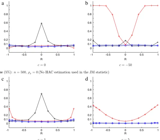
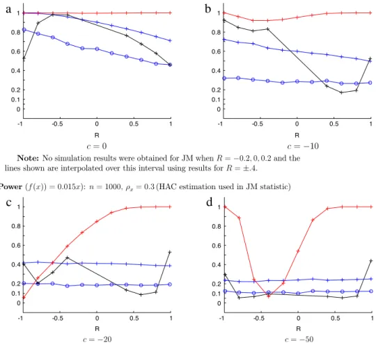
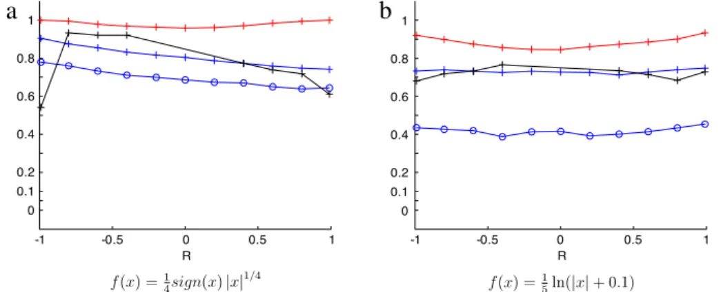
_t_FM_{) (see} _{Phillips and} Hansen, 1990;Phillips,1995) and theJansson and Moreira(2006,

hereafter JM), test statistic (R

ˆ

_β). We assume thatytis generated as

in(19)wherextis a (near) unit root process of the form(3)with

short memory innovations.5

When the regression function in (19) is linear it is readily shown that both test statistics attain a divergence rate of order

n. For f non-linear and locally integrable (but not integrable), the divergence rate is slower. Finally for f integrable the test statistics are bounded in probability and therefore inconsistent. These results are demonstrated inTheorem 3below.

Before presenting the results we introduce some notation. Define the covariance matrix

Ω

=

E







u2_t ∞



k=−∞ ut

v

t+k ∞



k=−∞

v

tut+k ∞



k=−∞

v

t

v

t+k







=



Ωuu Ωuv Ωvu Ωvv



.

(20)

For simplicity in the following presentation, we assume that

v

t is

i.i.d.6_{The subsequent results can be extended for the case where}

v

tis a linear process.7Next, consider the FM-OLS estimator in(18):

˜

β

=

n



t=1+ν y+_t xt−ν

−

1_n n



t=1+ν y+_t n



t=1+ν xt−ν n



t=1+ν x2_t−ν

−

1n



_n



t=1+ν xt−ν

2

,

˜

a

= ¯

y+

− ˜

β

¯

x

,

withy+_t

=

yt

− ˆ

v

tΩ

ˆ

_vv−1Ω

ˆ

vu,

v

ˆ

t

=

xt

− ˆ

ρ

xt−1. Here,Ω

ˆ

uu, Ω

ˆ

vuΩ

ˆ

vv are given by



ˆ

Ωuu

,

Ω

ˆ

vv

,

Ω

ˆ

vu



:=

1 n



_n



t=1+ν

ˆ

u2_t

,

n



t=2

ˆ

v

2 t

,

n



t=1+ν

ˆ

v

tu

ˆ

t



.

5 Note that the FM-OLS method ofPhillips(1995) and the J&M tests are both developed for unit root processes driven by short memory innovations.

6 In that caseΩ=E  u2_t utvt vtut v2t  .

7 In particular, the results of this section can be extended to the case wherevtis a

linear process (including SM, LM or AP cases). In order to obtain the limit properties of the parametric tests, whenvtis a linear process, we need to characterize the

pseudo-true limits of various long run variance estimators under functional form misspecification.Kasparis(2008) provides results of this kind for the SM case.

(8)

Next, define the pseudo-true values8 a∗

:=



1 0 Hf

(

G

(

r

))

dr

−

β

∗



1 0 G

(

r

)

dr

,

β

∗

:=



1 0 Hf

(

G

(

r

))

G

(

r

)

dr



1 0 G

(

r

)

2dr

,

β

∗∗

:=



1 0 G

(

r

)

dBu

(

r

)

−



1 0 G

(

r

)

dr



∞ −∞f

(

s

)

dsLG

(

1

,

0

)

+

Bu

(

1

)





1 0 G 2

(

r

)

dr

,

Ω∗ uu

:=



1 0



Hf

(

G

(

r

))

−

a∗

−

β

∗G

(

r

)

2

dr

,

Ω∗∗ uu

:=



Ω∗ uu

,

for

κ

f

(λ)

→ ∞

Ω∗ uu

+

Ωuu

,

for

κ

f

(λ)

=

1 Ωuu

,

for

κ

f

(λ)

→

0

,

andΩ+

=

Ω_uu

−

Ω_vv−1Ω_v2_u

,

whereBuis the Brownian motion limit of the partial sum process

ofut. The test statistics under consideration are

ˆ

tFM

=

˜

β







Ω

ˆ

+



n



t=1+_ν x2_t−ν

−

1_n



_n



t=1+_ν xt−ν

2



−1

,

and

ˆ

R_β

=

_

1

ˆ

ΩvvΩ

ˆ

+



1 n n



t=1+ν



xt−ν

−

1 n n



t=1+ν xt−ν



×



y+_t

− ˆ

β

xt−ν





,

whereΩ

ˆ

+

_{= ˆ}

_Ω uu

− ˆ

Ω_vv−1Ω

ˆ

_v2u,

β

ˆ

=





tx2t−ν

−

1 n



txt−ν

2



−1



tytxt−ν

−

1_n



tyt



txt−ν



.

Theorem 3. Suppose thatAssumption2.3SMholds with

v

ti.i.d. The fitted model is given by(18)and

{

yt

}

is generated by(19). Further, for f H-regular suppose that

√

n

κ

f

(

√

n

)

→ ∞

. Then

(a) Forf

(

x

)

(andxf

(

x

)

,f

(

x

)

2_{) H-regular and}

(i)

κ

f

(λ)

→ ∞

1

√

n

ˆ

tFM d

→



1 0 Hf

(

G

(

r

))

G

(

r

)

dr



Ω∗∗ uu



1 0 G

(

r

)

2dr

,

1

√

n

ˆ

R_β

→

d 1



ΩvvΩuu∗∗



1 0 G

(

r

)



Hf

(

G

(

r

))

−

β

∗G

(

r

)



dr

,

(ii)

κ

f

(λ)

=

O

(

1

)

1

κ

f

(

√

n

)

√

n

ˆ

tFM d

→



1 0 Hf

(

G

(

r

))

G

(

r

)

dr





Ω∗∗ uu

−

Ωvv−1Ωv2u

 

1 0 G

(

r

)

2dr

,

1

κ

f

(

√

n

)

√

n

ˆ

R_β

→

d

_

1 ΩvvΩuu∗∗

−

Ωv2u

×



1 0



G

(

r

)



Hf

(

G

(

r

))

−

β

∗G

(

r

)



dr

.

8 The quantitiesa∗, β∗, β∗∗andΩuu∗∗are the random limits of scaled versions

of the OLS coefficient and covariance estimators when the predictive regression is misspecified in terms of functional form.

(b) Forf

(

x

)

(andxf

(

x

)

) integrable

ˆ

tFM d

→

1

(Ω

+

)

1/2





Bu

(

1

)

−

σ

ξV

(

1

)Ω

−1 vvΩvu



−

cΩ_vv−1Ω_vu



1 0 G

(

r

)

2dr

1

/2



,

ˆ

R_β

→

d Rβ

−

√

β

∗∗ ΩvvΩ+



1 0 G

(

r

)

2dr

,

where Rβ

=

√

1 ΩvvΩ+



1 0 G

(

r

)

d



Bu

(

r

)

−

σ

ξV

(

r

)Ω

_vv−1Ωvu



−

cΩ_vv−1Ω_vu



1 0 G

(

r

)

2dr



.

Remarks.

(a) As indicated above, when the fitted model is correctly specified in terms of a linear functional form, parametric tests attain a divergence rate of orderni.e.

ˆ

tFM

,

R

ˆ

β

=

Op

(

n

) .

But when functional form misspecification is committed, The-orem 3suggests that parametric tests are either inconsistent or attain slower divergence rates. Divergence rates depend on the nature of the regression function. For locally integrable pre-dictive functions (that are not integrable) the test statistics di-verge at rates slower thann. For integrablegthe test statistics are bounded in probability and therefore the tests are incon-sistent. In particular, we have

ˆ

tFM

,

R

ˆ

β

=







Op



√

n



,

f H-regular

w

ith

κ

f

(λ)

→ ∞

Op



κ

f

(

√

n

)

√

n



,

f H-regular

w

ith

κ

f

(λ)

=

O

(

1

)

Op

(

1

),

f integrable

.

Note that forf polynomial H-regular the divergence rate is of orderOp

(

nς

)

with 0

< ς

≤

1

/

2.

(b) Forgintegrable we have the following outcomes.

(i) The limit distribution of the t

ˆ

FM statistic is identical to

that obtained under the null hypothesis. Therefore, in this case the asymptotic power of the test is identical to size. The simulation results presented in the subsequent section suggest that finite sample power is also close to size. (ii) The limit distribution of theR

ˆ

_βstatistic under the null

hy-pothesis is given byR_β. Under the alternative hypothesis an additional term features in the limit, viz.,

−

√

β

∗∗

ΩvvΩ+



1

0

G

(

r

)

2dr

.

(21)

This additional term is random and its sign is determined by the (random) pseudo true value

β

∗∗. Power is

corre-spondingly random, being influenced by the distribution of

(21), and may therefore be greater or less than the size of the test. The test is inconsistent in this case.

(c) IfΩuuis estimated by some HAC estimator, the divergence rates

of

ˆ

_t_FM_and_R

ˆ

_β_{will be adversely affected by the bandwidth term}

Mn(Mn

→ ∞

) employed in the HAC estimator.9In particular,

it can be shown that

ˆ

tFM

,

R

ˆ

β

=











Op



n Mn



,

Mn

κ

f

(

√

n

)

2

→ ∞

Op



κ

f

(

√

n

)

√

n



,

Mn

κ

f

(

√

n

)

2

=

O

(

1

)

Op

(

1

),

f integrable

.

9 IfΩvuorΩvvare estimated by HAC procedures, the divergence rates are the