econstor
www.econstor.eu
Der Open-Access-Publikationsserver der ZBW – Leibniz-Informationszentrum WirtschaftThe Open Access Publication Server of the ZBW – Leibniz Information Centre for Economics
Nutzungsbedingungen:
Die ZBW räumt Ihnen als Nutzerin/Nutzer das unentgeltliche, räumlich unbeschränkte und zeitlich auf die Dauer des Schutzrechts beschränkte einfache Recht ein, das ausgewählte Werk im Rahmen der unter
→ http://www.econstor.eu/dspace/Nutzungsbedingungen nachzulesenden vollständigen Nutzungsbedingungen zu vervielfältigen, mit denen die Nutzerin/der Nutzer sich durch die erste Nutzung einverstanden erklärt.
Terms of use:
The ZBW grants you, the user, the non-exclusive right to use the selected work free of charge, territorially unrestricted and within the time limit of the term of the property rights according to the terms specified at
→ http://www.econstor.eu/dspace/Nutzungsbedingungen By the first use of the selected work the user agrees and declares to comply with these terms of use.
zbw
Leibniz-Informationszentrum Wirtschaft Leibniz Information Centre for Economics Hafner, Christian M.; Herwartz, HelmutWorking Paper
Testing for Causality in Variance using
Multivariate GARCH Models
Economics working paper / Christian-Albrechts-Universität Kiel, Department of Economics, No. 2004,03
Provided in cooperation with:
Christian-Albrechts-Universität Kiel (CAU)
Suggested citation: Hafner, Christian M.; Herwartz, Helmut (2004) : Testing for Causality in Variance using Multivariate GARCH Models, Economics working paper / Christian-Albrechts-Universität Kiel, Department of Economics, No. 2004,03, urn:nbn:de:101:1-200911033770 , http://hdl.handle.net/10419/21980
Economics Working Paper
No 2004-03
Testing for Causality in Variance using
Multivariate GARCH Models
Testing for Causality in Variance using Multivariate
GARCH Models
Christian M. Hafner
∗Helmut Herwartz
†March 17, 2004
Abstract
Tests of causality in variance in multiple time series have been proposed recently, based on residuals of estimated univariate models. Although such tests are applied frequently little is known about their power properties. In this paper we show that a convenient alternative to residual based testing is to specify a multivariate volatil-ity model, such as multivariate GARCH (or BEKK), and construct a Wald test on noncausality in variance. We compare both approaches to testing causality in vari-ance in terms of asymptotic and finite sample properties. The Wald test is shown to have superior power properties under a sequence of local alternatives. Furthermore, we show by simulation that the Wald test is quite robust to misspecification of the order of the BEKK model, but that empirical power decreases substantially when asymmetries in volatility are ignored.
Keywords: causality, multivariate volatility, local power JEL Classification: C22, C52
∗Econometric Institute, Erasmus University Rotterdam, P.O.B 1738, 3000 DR Rotterdam, The
[email protected](corresponding author)
†Institut f¨ur Statistik und ¨Okonometrie, Christian Albrechts Universit¨at zu Kiel, Ohlshausenstr.
1
Introduction
Causal relationships in systems of economic time series variables are often defined accord-ing to forecastaccord-ing principles exploitaccord-ing the idea that a cause must precede its effect in time. Tests of Granger causality (Granger (1969), Granger (1980), Granger (1988)) have become a standard step when analyzing linear systems of time series. In light of a still growing interest in dynamics of financial data recent work on causality also addresses the issue of second order causality and/or causality in variance (Granger, Robins and Engle (1986), Cheung and Ng (1996), Comte and Liebermann (2000)).
For testing the hypothesis of noncausality in variance two approaches have been fol-lowed in the literature. On the one hand two step methodologies have been introduced which concentrate on the cross correlation function (CCF) of univariate residual estimates. Building upon tests on causality in mean (Haugh (1976), Pierce and Haugh (1977)) Che-ung and Ng (1996) follow these lines to infer on cross sectional dependence of squared GARCH innovations. Kanas and Kouretas (2002) employ the CCF-test introduced by Cheung and Ng (1996) to detect volatility spillovers between official and black currency markets.
Alternatively, causality in variance is often diagnosed by means of (Quasi) Maximum-Likelihood ((Q)ML) methods which utilize a parametric specification of volatility dynam-ics of systems of financial data. In particular, the BEKK form of the multivariate GARCH model (Engle and Kroner, 1995) allows to establish a one-to-one relation between non-causality in variance and particular testable zero restrictions imposed on the parametric model. One of the arguments of Cheung and Ng (1996) against using specifications of multivariate GARCH models was that a rigorous proof of asymptotic QML theory in the multivariate GARCH framework was still missing. This argument, however, is no longer valid after recent progress on the theoretical side, e.g., by Comte and Lieberman (2003). Comte and Lieberman (2000) provide a unified treatment of first and second order causality in the framework of VARMA models with multivariate GARCH error terms. The BEKK model is widely used to test causal relationships between financial time series (see e.g. Hafner and Herwartz (1998), Herwartz and L¨utkepohl (2000), Caporale, Spittis and Spagnolo (2002)). It is worthwhile to mention that both approaches to inference on causality, the two step and the ((Q)ML) methodology, have not yet been compared in terms of their empirical properties.
In this paper we pick up the definitions of causality in variance and linear causality in variance given in Comte and Lieberman (2000) for the multivariate GARCH model and relate it to the notions of strong, semi-strong and weak GARCH processes going back to Drost and Nijman (1993). We give sufficient and necessary conditions for (lin-ear) noncausality in variance and derive testable parametric restrictions covering these restrictions. We provide a local power analysis and a Monte Carlo study to investigate the relative performance of the CCF-test and Wald-type tests derived from asymptotic (Q)ML theory. The robustness of the latter methodology under misspecification of the (quasi) log-likelihood function is also addressed.
method-ological framework for our analysis, the multivariate GARCH model and its VARMA representation. In Section 3 causality in variance and linear causality in variance are defined and competing tests of the null hypothesis of higher order noncausality are mo-tivated. A local power investigation compares two approaches to causality testing which are frequently used, the CCF and the Wald test. A Monte Carlo study in Section 4 is provided to assess the finite sample properties of alternative tests on noncausality in variance. Section 5 briefly summarizes our main results and underscores their scope for empirical multivariate volatility modelling. Proofs and details of implementing the Wald test are given in Appendices A and B.
2
Multivariate GARCH Models
Let us first introduce the terminology of weak, semi-strong and strong multivariate GARCH models, analogously to the univariate case. Later we will define causality in variance con-cepts that naturally apply these alternative notions of GARCH models.
Definition 1 (Multivariate GARCH) Let εt denote a stochastic vector process with K components and E[εt | Ft−1] = 0. Now define a positive definite and symmetric matrix
Ht such that ht=vech(Ht) has the representation ht =ω+ q X i=1 Aiηt−i+ p X j=1 Bjht−j, (1)
where ω = vech(Ω), ηt =vech(εtε0t) and Ω, Ai, Bj, are K∗×K∗ parameter matrices with K∗ =K(K+ 1)/2. Then we say that ε
t is a
1. strong multivariate GARCH(p, q) process, if ξt = Ht−1/2εt is an i.i.d. process with
mean zero and variance the identity matrix,
2. semi-strong multivariate GARCH(p, q) process, if Var(εt | Ft−1) = Ht,
3. weak multivariate GARCH(p, q) process, if ht is the best linear predictor of ηt in
terms of a constant and lagged values of ηt, that is
ht=P(ηt| Ht−1) = [P(ηt,1 | Ht−1), . . . , P(ηt,K∗ | Ht−1)]0
where Ht denotes the Hilbert space spanned by a constant and ηt−τ,1, . . . , ηt−τ,K∗,
τ ≥0.
A strong multivariate GARCH(p, q) process is also semi-strong, and a semi-strong multivariate GARCH(p, q) process is also weak, which justifies the terminology.
To establish the analogy to VARMA models, rewrite the process (1) as
ηt=ω+ max(Xp,q) i=1 (Ai +Bi)ηt−i− p X j=1 Bjut−j+ut, (2)
withut =ηt−ht and where we setAq+1 =. . .=Ap = 0 ifp > q andBp+1 =. . .=Bq = 0
if q > p. It now depends on the properties of ut if we can consider (2) as a VARMA
process.
Assumption 1 The covariance matrix of ut, Σu = E[utu0t], is assumed to be finite and
positive definite.
For the case of a strong multivariate GARCH(p, q) model with spherical distribution ofξt,
necessary and sufficient conditions for Assumption 1 to hold are given in Hafner (2003). We now have the following result.
Lemma 1 Under Assumption 1, if {εt} is
1. strong or semi-strong multivariate GARCH(p, q), then {ut} in (2) is a martingale
difference process.
2. weak multivariate GARCH(p, q), then {ut} is weak white noise in the sense that
E[ut] = 0, E[utu0s] = 0, ∀t6=s, and E[utu0t] = Σu <∞.
As a result of this lemma, {ηt} in (2) follows a VARMA(max(p, q), p) process under
Assumption 1. In the case of strong and semi-strong multivariate GARCH, this VARMA process characterizes the conditional mean ofηt, whereas in the case of weak multivariate
GARCH, it characterizes the best linear predictor of ηt in terms of lagged values of ηt.
Thus, when defining causality concepts we will have to distinguish between concepts that are based on the conditional mean and concepts based on best linear predictors.
In the following we will assume covariance stationarity of the process εt.
Assumption 2 All eigenvalues of the matrix Pmax(i=1 p,q)(Ai +Bi) have modulus smaller
than one.
The multivariate GARCH(p, q) process εt is covariance stationary if and only if
Assump-tion 2 holds, see e.g. Engle and Kroner (1995). In that case, the components of the unconditional covariance matrix Σ = Var(εt) are given by
σ = vech(Σ) = IK∗− max(Xp,q) i=1 (Ai+Bi) −1 ω. (3)
Under Assumption 2, one obtains the VMA(∞) representation from the VARMA
representation (2), ηt =σ+ ∞ X i=0 Φiut−i, (4)
where the K∗×K∗ matrices Φ
i can be determined recursively by Φ0 =IK∗,
Φi =−Bi+ i
X
j=1
see L¨utkepohl (1993, pp. 220).
In practice it is often easier to work with the so-called BEKK model of Engle and Kroner (1995), which is a special case of the vec model. The BEKK model involves less parameters to be estimated and ensures positive definiteness ofHtunder weak conditions.
In its general form, the BEKK(p, q, S) model can be written as
Ht=CC0 + S X s=1 q X i=1 A∗ siεt−iε0t−iA∗0si+ S X s=1 p X i=1 B∗ siHt−iBsi∗0, (6)
where C is a lower triangular matrix and A∗
si and Bsi∗ are K ×K parameter matrices.
For illustrative purposes, we will only consider the case p=q =S = 1, which is also the mostly applied model order. Thus, the model simplifies to
Ht=CC0+A∗εt−1εt0−1A∗0+B∗Ht−1B∗0, (7)
with
ϑ= (vech(C)0,vec(A∗)0,vec(B∗)0)0 (8)
being a K(5K+ 1)/2-dimensional parameter vector. Note that each BEKK model has a corresponding unique vec representation, but not vice versa, see Engle and Kroner (1995).
3
Causality Tests
In order to define causality concepts for the variance of a vector process εt, we make in
the following two assumptions that simplify the presentation and allow us to focus on the issue of inference for causality. The first assumption is that the conditional mean is zero, i.e., E[εt | Ft−1] = 0. Without this assumption, there would be a difference between a
concept that corrects for the mean using all available information and one that corrects for the mean using only the information of the variable that is to be caused by the others. The first notion was introduced by Granger, Robins and Engle (1986), and the second one by Comte and Lieberman (2000). Under the assumption E[εt | Ft−1] = 0, however,
both notions are equivalent.
The second simplifying assumption concerns the number of sub-groups of the vectorεt.
We assume that there are only two sub-groups, and we investigate concepts of causality between these two groups. As is well known, e.g. from Dufour and Renault (1998), in such setups it suffices to investigate the causality horizon of one period. If there is noncausality at horizon one, then there is noncausality at every horizon. If there were more sub-groups of the vectorεt, and we were investigating the causality between the first
two sub-groups, say, then there could be causality at larger horizons even though there may not be causality at horizon one. The intuitive reason is that there may be a causality chain going from the causing sub-group to a third sub-group, and then in a later period from this third sub-group to the sub-group to be caused. Thus, our restriction to only two sub-groups means that we can restrict our attention to a horizon of one period, which is notationally convenient. About all results of Dufour and Renault (1998) apply in our
setting as well, so that we only discuss the simple case here and all extensions follow by analogy.
First, define the index sets I = (i1, . . . , ik) and J = (j1, . . . , jK−k), where I ∪ J =
(1, . . . , K) andI∩J =∅. We will investigate the issue whether the variables indexed byJ cause the variables indexed by I. We define the sub-vectors of εt byεIt = (εt,i1, . . . , εt,ik)0
and εJt = (εt,j1, . . . , εt,jK−k)
0, and let ηI
t = vech(εItεI0t ), which is a vector of length k∗ = k(k + 1)/2. The σ-algebras generated by εI
s and εJs , s ≤ t, are denoted by FtI and
FJ
t , respectively. Moreover, denote by HIt the Hilbert space spanned by the variables ηI
s,1, . . . , ηs,kI ∗,s ≤t.
Now, similar to Comte and Lieberman (2000), we define causality in variance and linear causality in variance.
Definition 2 We say that
• εJt does not cause εI
t in variance, denoted by εJt V 9εI t, if Var(εI t | Ft−1) = Var(εIt | FtI−1) • εJ
t does not cause εIt linearly in variance, denoted by εJt LV
9 εI
t, if P(ηIt | Ht−1) = P(ηtI | HtI−1)
3.1
The CCF test
Based on squared residuals ˆξ2
i,t =ε2i,t/σˆi,t2 , where ˆσi,t2 is the estimated conditional variance
ofεi,t using univariate GARCH, Cheung and Ng (1996) introduce a portmanteau statistic
to test the null hypothesis of noncausality in variance,
H0 :εj,t 9V εi,t, ∀i∈ I,∀j ∈ J.
The test statistic builds upon sample cross correlations and reads as
Pm=T m X l=1 r2 ij,l, i∈ I, j ∈ J, (9) where rij,l= cij,l √c ii,0cjj,0 , cij,l = 1 T T X t=1 (ξ2 i,t −ξi2)(ξj,t2 −l−ξj2), and where ξ2 i =T−1 PT t=1ξi,t2 .
In practice, the choice ofm should allow to cover the highest potential lag of causality in variance. Cheung and Ng (1996) prove that under consistent estimation of the uni-variate GARCH parameters, Pm follows asymptotically a χ2(m)-distribution under the
null hypothesis. Analogous statistics can be defined for testing the hypothesis of bidirec-tional causality. Also, in small samples one can use modified portmanteau statistics in the standard manner.
The CCF test has the appealing feature to be easily computable. A drawback, however, is that the ordermhas to be determined. Ifmis chosen too small, one may miss causalities at higher lags, if it is chosen too large, the degrees of freedom increase and, hence, the power of the test decreases. We will show later that the CCF test has very poor power properties if the alternative is multivariate GARCH, irrespective of the choice ofm.
3.2
A pseudo likelihood ratio statistic
The CCF test estimates univariate GARCH models and then tests for cross-correlations between standardized (squared) residuals. If there are only two series, it can be thought of estimating the model under the null hypothesis of no bi-directional causality, so that it is in the spirit of Lagrange multiplier statistics. In the next section we are going to discuss Wald type statistics. It is also possible to consider statistics in the spirit of likelihood ratio statistics, where both univariate and multivariate models are estimated. Likelihood ratio tests of causality in linear VARMA type models have been introduced by Geweke (1982) and extended to multivariate GARCH models by Hafner (2003).
To define the test statistic, consider a bivariate GARCH process and its VARMA representation (2), where the error termuthas, by Assumption 1, finite covariance matrix
Σu. Having a sample of T observations and considering causality in variance from ε2t to ε1t, we may alternatively estimate a univariate GARCH model of appropriate order for ε1t, obtain its ARMA representation and the corresponding residual variance,σ2v say. Now
the statistic is given by
LR =T log σv2
Σu,11
. (10)
In VARMA models with Gaussian errors, (10) is the usual likelihood ratio statistic. The problem in multivariate GARCH models is that the errors of the VARMA representation (2) are not Gaussian and typically highly skewed. Thus, (10) is not the true LR statistic and will be biased if compared with a χ2 distribution. Nevertheless, it might be useful for
descriptive purposes. We have used bootstrapped versions of the statistic (10) to correct for the size, but the power turned out to be equally poor as for the CCF test. Therefore, we do not report these results in this paper to economize on space.
3.3
Tests based on multivariate GARCH models
Noncausality in variance amounts to certain zero restrictions of the matrices Ai and Bj
in (1). To find these restrictions, we first define the index
kK ij =i+ (j −1) µ K − j 2 ¶ (11)
for i, j ∈ I ∪ J and i ≥ j, which is the position of the (i, j)-th element of a (K ×K) symmetric matrix M in the vector vech(M). Recall that vech(M) containsK∗ =K(K+
1)/2 elements. Moreover, we define the index sets I∗ ={kK
ij |i, j ∈ I} (12)
and
J∗ ={1, . . . , K∗} \ I∗. (13)
This notation at hand, we can now give conditions for noncausality in variance. Let us consider the following two conditions,
[Φn]ij = 0, ∀n ≥1, ∀i∈ I∗, ∀j ∈ J∗, (14)
and
[Aa]ij = 0, a = 1, . . . , q, [Bb]ij = 0, b = 1, . . . , p, ∀i∈ I∗, ∀j ∈ J∗. (15)
Theorem 1 If εt is a weak multivariate GARCH process, then condition (14) is
neces-sary and sufficient and condition (15) is sufficient for εJt LV9 εI
t. If εt is a semi-strong
multivariate GARCH process, then each one of conditions (14) and (15) is sufficient for
εJ
t V
9εI
t.
Proof: see Appendix.
The first part of Theorem 1 is well known, see e.g. L¨utkepohl (1993, p. 236f.). Unlike in the first part, no equivalence between Condition (14) and variance noncausality can be established in the second part. The reason for this is that, if εt is a semi-strong
multivariate GARCH process, then a subprocess is only weak GARCH, see Nijman and Sentana (1996). Thus, the conditional expectation of a subprocess of ηt may not be a
linear function of laggedηt, and the restrictions that variance noncausality implies become
impossible to express in terms of the moving average coefficients Φn.
Turning to the testing problem, note that Condition (14) is infeasible to test due to the large number of coefficient matrices to be tested. We therefore focus attention on testing Condition (15), but according to Theorem 1 it is only a sufficient condition for variance noncausality, even in the linear causality sense. Fortunately, for the often used multivariate GARCH(1,1) model,
ht =ω+Aηt−1+Bht−1, (16)
where Condition (15) simplifies to
[A]ij = 0, [B]ij = 0, ∀i∈ I∗, ∀j ∈ J∗, (17)
it turns out that both conditions are equivalent under an additional assumption.
Lemma 2 In the multivariate GARCH(1,1) model (16), ifAis invertible, then conditions (14) and (17) are equivalent.
Proof: see Appendix.
As a consequence of this lemma, if A is invertible, then testing (17) is equivalent to testing variance noncausality and linear variance noncausality, respectively. Note the difference to VARMA(1,1) models where (17) is only a sufficient condition for noncausality, see e.g. L¨utkepohl (1993, p. 236f.). The reason for this difference is the particular parameter structure of GARCH models, that is, the sum of the autoregressive parameter matrix (A+B) and the moving average matrix (−B) is just equal toA, giving Φ1 =A, so
thatAdirectly inherits the properties of Φ1. In the VARMA(1,1) model, Φ1 is equal to the
sum of the autoregressive and moving average parameter matrices, so that a restriction of Φ1 does not necessarily convey to each one of these.
Since Condition (17) in weak GARCH(1,1) models is not only sufficient but also nec-essary for linear noncausality in variance, testing this condition under the null hypothesis of no linear causality in variance should provide correct Type I and Type II errors. It is also likely to have more power than alternative tests that are based on only necessary conditions for noncausality, such as the CCF test of Cheung and Ng (1996).
In the following we will only discuss testing in GARCH(1,1) models, so that we will only consider tests of Condition (17). It is now straightforward to define a test statistic that tests the zero restrictions on A and B. Let us first define the following restriction matrix.
Definition 3 Let R˜ be a matrix of dimension k∗(K∗−k∗)×(K∗)2, of rank k∗(K∗−k∗).
The (r, τ) element of R˜ is defined by
˜ Rr,τ = ½ 1, τ =smn 0, τ 6=smn where r =m+ (n−1)k∗, s mn =im+ (jn−1)K∗, im ∈ I∗, jn ∈ J∗, and m = 1, . . . , k∗, n= 1, . . . , K∗ −k∗.
Each row of ˜R contains a one at the i+ (j−1)K∗-th position, where i∈ I∗ and j ∈ J∗,
and zeros elsewhere. Appendix B gives some examples how to find the restriction matrix ˜
R.
The null hypothesis of no causality can be written as
H0 :Rθ= 0 (18)
with θ = (ω0,vec(A)0,vec(B)0)0, and
R = [0(k∗(K∗−k∗)×K∗),R,˜ R˜]
If the BEKK(1,1,1) model (7) model is used, then equivalent conditions can be found that involve less equations. To formalize this idea, let us define the restriction matrix ˜Q
Definition 4 Let Q˜ be a matrix of dimension k(K−k)×(K)2, of rank k(K−k). The (r, τ) element of Q˜ is defined by ˜ Qr,τ = ½ 1, τ =smn 0, τ 6=smn where r = m+ (n−1)k, smn = im + (jn −1)K, im ∈ I, jn ∈ J, and m = 1, . . . , k, n= 1. . . , K −k.
The null hypothesis of no causality in the BEKK(1,1,1) model can now be written as
H0 :Qϑ= 0 (19)
with ϑ given by (8), and where
Q= [0(k(K−k)×K),Q,˜ Q˜].
The following theorem states the equivalence of the conditions (18) and (19).
Theorem 2 If the multivariate GARCH model has the BEKK(1,1,1) representation (7), then the noncausality conditions (18) and (19) are equivalent.
Proof: see Appendix.
Note that, although equivalent, condition (19) only involves k(K −k) equations as opposed to the (k∗(K∗ −k∗) equations of condition (18). In standard likelihood based
tests, the reduction in degrees of freedom may therefore result in more power if a BEKK model is used instead of a vec model, provided the data are well described by a BEKK model. Essentially, many conditions of (18) are redundant and just implied by (19). For example, if K = 2 andk = 1, then (18) has two equations and (19) only one.
Suppose now that we haveT observations,ε1, . . . , εT.We assume in the following that
the true process is known to belong to the BEKK class, for which asymptotic theory of estimation and inference is well developed, see Comte and Lieberman (2003). Denote a consistent estimator of the true parameter vectorϑ0 by ˆϑand assume that its asymptotic
distribution is given by √
T(ϑb−ϑ0)−→L N(0,Σϑ), (20)
with some positive definite and symmetric matrix Σϑ. Assume also that a consistent
estimate for Σϑ is given by Σbϑ. For example, if QML estimation is used, then (20) holds
under regularity conditions listed by Comte and Lieberman (2003), and Σϑ is given by
Σϑ=S−1DS−1, where D= E " ∂lt(ϑ) ∂ϑ ∂lt(ϑ) ∂ϑ0 ¯ ¯ ¯ ¯ ϑ0 # , S =−E " ∂2l t(ϑ) ∂ϑ∂ϑ0 ¯ ¯ ¯ ¯ ϑ0 # ,
with lt(ϑ) =− K 2 ln(2π)− 1 2ln|Ht(ϑ)| − 1 2ε 0 tHt−1(ϑ)εt. (21)
Hafner and Herwartz (2003) provide expressions for D and S and of their estimates. For significance testing Hafner and Herwartz (2003) show that making use of analytical expressions for Σϑ is by far superior to using numerical derivatives in terms of empirical
size and power estimates.
We propose the following standard Wald statistic for testing the hypothesis (19),
WT =T(Qϑˆ)0(QΣbϑQ0)−1(Qϑˆ). (22)
Using (20) and Proposition C.4 of L¨utkepohl (1993), the asymptotic distribution of the Wald statistic is given by
WT −→L χ2k(K−k).
An analogous statistic can be defined for the vec model based on the null hypothesis (18), provided that conditions for asymptotic normality of estimators hold, which is as yet unknown. Note that the degrees of freedom of the Wald statistic for the vec model would be k∗(K∗−k∗).
3.4
A power comparison
We now investigate the asymptotic power of the Wald and the CCF tests under a sequence of local alternatives. To ensure that all asymptotic results are valid we still assume that the model is known to belong to the BEKK class. Consider the parameter vector
ϑ0T =ϑ0+δ/
√
T
where ϑ0 is the parameter vector under the null hypothesis and δ is a fixed vector of the
same length as ϑ0. Under local alternatives, we have the asymptotic distribution
√
T(ϑb−ϑ0T) =
√
T(ϑb−ϑ0) +δ −→L N(δ,Σϑ). (23)
As a consequence, the Wald statistic in (22) has the following asymptotic distribution under local alternatives,
WT −→L χ2k(K−k)(λ),
i.e., a noncentral χ2 distribution with k(K −k) degrees of freedom and noncentrality
parameter λ given by
λ= (δ0Q0)(QΣϑQ0)−1Qδ.
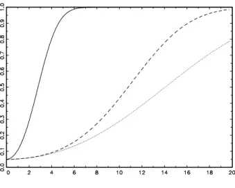
One can now derive the asymptotic power of WT as a function of δ. If only one element
of δ is different from zero, then one can plot the asymptotic power as a function of this element, as done in Figure 1 for the process defined in the next section.
Next, we can derive the asymptotic power of the CCF test under a sequence of local alternatives ϑ0T that characterizes a multivariate GARCH alternative. We obtain, using
a Taylor expansion around ϑ0,
√ Trˆij,l(ϑ0T) = √ Trˆij,l(ϑ0) + ∂rˆij,l ∂ϑ0 ¯ ¯ ¯ ¯ ϑ0 δ+Op(T−1/2).
Assuming consistency of correlation estimates, i.e., plim ˆrij,l(ϑ0) = rij,l(ϑ0), we obtain for
the vector of correlations up to lag m, √ Trˆm ij(ϑ0T)−→L N Ã ∂rm ij ∂ϑ0 ¯ ¯ ¯ ¯ ϑ0 δ, Im ! . where rm
ij = (rij,1, . . . , rij,m)0. Hence, the CCF statistic Pm =T
m
X
l=1
rij,l2 −→L χ2m(λ)
has, asymptotically, a noncentralχ2 distribution with m degrees of freedom and
noncen-trality parameter λ given by
λ=δ0 ∂r m0 ij ∂ϑ ¯ ¯ ¯ ¯ ϑ0 ∂rm ij ∂ϑ0 ¯ ¯ ¯ ¯ ϑ0 δ.
The derivative can be calculated numerically. We generate 500 bivariate diagonal BEKK processes withT = 10000, estimate univariate GARCH processes, obtain residuals
ˆ
ξ1,t and ˆξ2,t and calculate correlations ˆrijm. The same is done for a bivariate BEKK process
with lower left element of the A∗ matrix changed to -0.01 and 0.01, and the mean of the
corresponding derivatives of ˆrm
ij is a good approximation of∂rijm/∂ϑ0. For the BEKK(1,1,1)
process (7) with parameters specified in Section 4, the asymptotic power function of the CCF test is depicted in Figure 1 together with the corresponding function for the Wald test, assuming Gaussian innovations. Clearly, the Wald test has uniformly higher power in a neighborhood of ϑ0. We get a very similar picture in Figure 2 when assuming
multivariatet8 distributed innovations, where the power drops slightly for both the Wald
and the CCF tests.
4
Finite sample performance
The following Monte Carlo investigation is thought to shed light on the empirical per-formance of two strategies for inference on noncausality in variance. We compare the empirical properties of the Wald statistic in (22) on the one hand and of the CCF test introduced by Cheung and Ng (1996) on the other hand.
4.1
The Monte Carlo design - Wald vs. CCF
To illustrate the empirical size properties of competing approaches to test noncausality in variance we simulate bivariate GARCH-processes of the BEKK-form (S =p=q = 1) according to the following choice of parameter matrices:
C = µ 1.10 0.00 0.30 0.90 ¶ , A∗ = µ 0.25 0.00 0.00 0.25 ¶ , B∗ = µ 0.90 0.00 0.00 0.90 ¶ . (24) We test three null hypotheses. The first null hypothesis states that there is no causality in variance in the system at all. The second and third null hypothesis formalize that
ε1t does not cause ε2t in variance and vice versa. In summary we test the following null
hypotheses:
H0(1) : ε1t 9V ε2t, ε2t9V ε1t, H0(2) : ε1t 9V ε2t,
H0(3) : ε2t 9V ε1t.
We also provide empirical power estimates for the cases when testingH0(1) orH0(2). Under the alternative hypotheses we choose the parameter matrices A∗ and B∗ as
A∗ = µ .250 .000 .025 .250 ¶ , B∗ = µ .900 .000 .025 .900 ¶ . (25) To indicate the relative performance of exact ML inference on the one hand and the QML methodology on the other hand we draw underlying innovations alternatively from a bivariate Gaussian distribution or as standardized and independent innovations from a t−distribution with 8 degrees of freedom. Note that under Gaussian innovations estimating the asymptotic covariance matrix as ˆΣϑ = ˆS−1DˆSˆ−1, could be inefficient in
small samples (Hafner and Herwartz (2003)). Under conditional leptokurtosis making use of a covariance estimator ˆΣϑ = ˆD−1 will result in size distortions. We consider sample
sizes T = 1000,2000,4000,8000. The nominal significance level for all performed tests is
α= 0.05. Each process is generated 2000 times.
4.2
Simulation results
Table 1 shows empirical rejection frequencies for the Wald statistics implemented alter-natively with covariance estimators ˆD−1 (W1) and ˆS−1DˆSˆ−1(W2). Overall the empirical
size estimates are larger than their nominal counterparts, and often exceed the latter significantly at the 5% level even in large samples (T = 8000). Empirical size esti-mates are in almost any case somewhat larger when testing on overall noncausality (H0(1)) in comparison to testing on unidirectional noncausality (H0(2), H0(3)). Under leptokurtic (standardized t−distributed) innovationsξt, W1 shows huge size distortions whereas the
size increases (T = 8000). Moreover, under conditional normality estimating the asymp-totic covariance matrix as ˆΣϑ= ˆS−1DˆSˆ−1 yields higher size estimates in comparison with
W1. For instance, testing H0(1) under conditional normality in samples of size T = 1000 obtains empirical rejection frequencies of ˆα = 0.077 and ˆα = 0.121 for W1 and W2, re-spectively. Relative to the nominal level of α = 0.05 it is evident, that the choice of the robust covariance estimator may go at the cost of size distortions.
With respect to power properties testing overall noncausality (H0(1)) turns out to be less effective than unidirectional testing (H0(2)) when actuallyε1tis causingε2tand ε2,t 9V ε1,t.
Under conditional normality (conditional leptokurtosis), for instance, W1 (W2) delivers empirical rejection frequencies which are up to 9% higher when testing H0(2) instead of
H0(1).
Table 2 displays selected simulation results for the CCF-test, namely size estimates for the case T = 1000 and power estimates for samples of size T = 8000 under both, conditional normality and leptokurtosis. Results are shown for alternative test orders (m). Apparently the size properties obtained from CCF are close to the nominal level and therefore superior relative to the performance of the Wald statistics. In terms of power, however, the CCF approach performs rather poor. For example, testing under Gaussian innovations in samples of size T = 8000 the most favorable rejection frequency obtained for the CCF-test is 15.75% which is by far inferior to the Wald test delivering empirical power estimates of about 80.0%.
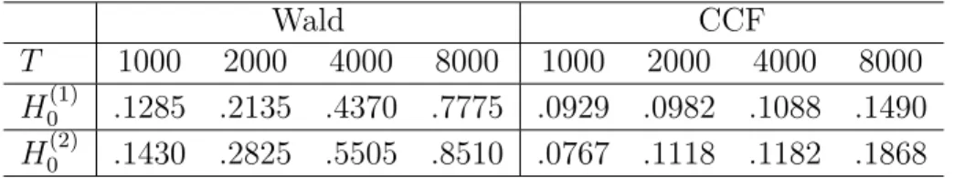
Given that W1 and W2 tend to reject under the null hypothesis more often than CCF it is sensible to compare size adjusted power estimates. For this purpose Table 3 displays rejection frequencies obtained when testing H0(1) and H0(2) for the Gaussian model with ε1t causing ε2t in variance. Size adjustment is here achieved by tuning the
nominal level of the CCF test such that under the null hypothesis both test procedures, the Wald and the CCF, give identical empirical size estimates. Apparently, W1 clearly outperforms the CCF-test after size adjustment. In samples with T = 4000 orT = 8000 size adjusted power estimates of W1 are up to five times larger than the corresponding estimates obtained for the CCF-test. Note that the latter result is particularly important for practical purposes. Adopting the CCF approach to test for causality in variance will often fail to uncover causal relationships and will thereby tend to preclude multivariate volatility models allowing cross equation dynamics, as e.g. the BEKK-model.
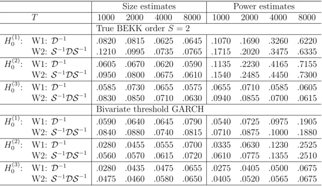
4.3
The Wald test under misspecification of the DGP
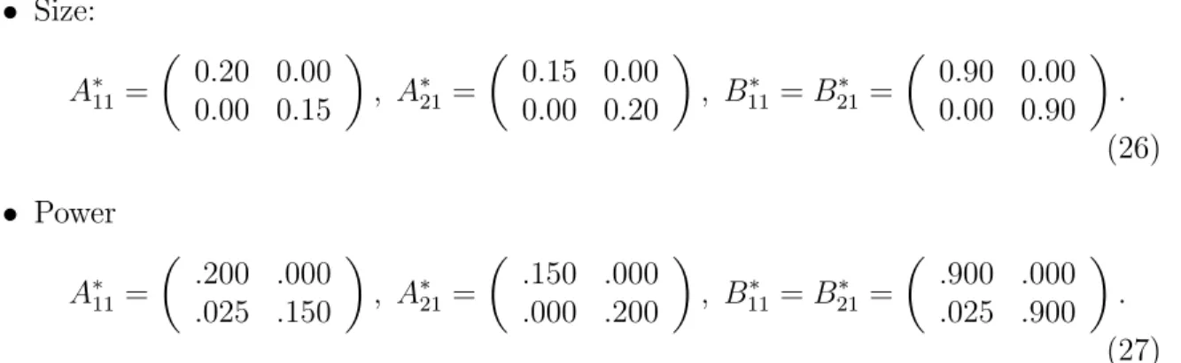
As outlined before the Wald statistic is obtained from QML-estimation of the multivariate GARCH process. To indicate the impact of misspecification of the underlying DGP and, thus, of the (quasi) log-likelihood function we follow two lines. First, we estimate BEKK models of order S = p = q = 1 when the true DGP has a higher BEKK order, namely
S = 2. In this case we use the following parameter choices to evaluate size and power properties, respectively:
• Size: A∗11= µ 0.20 0.00 0.00 0.15 ¶ , A∗21= µ 0.15 0.00 0.00 0.20 ¶ , B∗11=B21∗ = µ 0.90 0.00 0.00 0.90 ¶ . (26) • Power A∗11= µ .200 .000 .025 .150 ¶ , A∗21= µ .150 .000 .000 .200 ¶ , B∗11=B21∗ = µ .900 .000 .025 .900 ¶ . (27) Second, we estimate symmetric multivariate GARCH models in case the true under-lying DGP exhibits an asymmetric impact of current (co)variances to lagged innovations. For this purpose we use a bivariate threshold GARCH specification as in Hafner and Herwartz (1998) or Herwartz and L¨utkepohl (2000) generalizing the univariate process introduced by Glosten, Jaganathan and Runkle (1993). Formally the asymmetric DGP is specified by means of a state dependent parameter matrixAe∗
11replacing the corresponding
parameters in (6). The latter is chosen as e
A∗
11 =A∗11I(ε1,t−1 <0) +A∗21I(ε2,t−1 <0), (28)
whereI(·) is an indicator function andA∗
11andA∗21are given in (26) and (27) for assessing
size and power properties, respectively. With respect to the choice of the matrix B∗ 11 the
asymmetric process is identical to the symmetric specification with parameters given in (24) and (25).
4.4
QML under misspecification - Simulation results
Table 4 shows empirical size and power estimates for QML inference under conditional normality. Empirical size estimates of both Wald tests, W1 and W2, are almost unaffected when modelling a process parameterized with (26) under misspecification of the order parameterS. When testingH0(1)orH0(2)under the alternative of causal relations, however, underestimating the BEKK order involves losses in terms of power. For instance, in case T = 8000 testing H0(2) in presence of causal relationships yields empirical rejection frequencies for W1 of .851 and .716 if the BEKK order of the underlying model is S = 1 and S = 2, respectively. Under the null hypothesis W1 shows an empirical size of 5.09% for both (true) BEKK orders underlying the DGP. In comparison with misspecifying the BEKK order, ignoring the potential of an asymmetric response of volatility with respect to the sign of lagged error terms εt−1 involves slightly higher empirical size distortions
under the null hypothesis but huge power losses under the alternative. For example, employing the symmetric BEKK model to test on overall noncausality (H0(1)) by means of W1 and in case T = 8000 yields empirical size and power estimates of 6.35% and 77.75% (7.9% and 19.05%) if the true DGP exhibits a symmetric (asymmetric) impact of εt−1 on
5
Conclusions
We formalize the concepts of strong, semi strong, and weak multivariate GARCH. Using the general vec representation of this model and building on Comte and Lieberman (2000) we prove sufficiency or necessity of particular parameter restrictions for noncausality in variance (linear causality in variance). Two approaches to testing for causality in variance, namely the CCF test introduced by Cheung and Ng (1996) and a Wald test based on (Q)ML theory are discussed. Evaluating the asymptotic local power properties we find that the CCF test is inferior.
A Monte Carlo investigation indicates that the CCF test has more favorable empirical size properties in comparison with the Wald test. The former test, however, is also characterized by a severe shortfall in terms of empirical power. As a particular drawback of the (Q)ML based approach one may regard the necessity of a (potentially misspecified) parametric model to formalize the log likelihood function. Our results indicate that ignoring an asymmetric impact of volatility on lagged innovations will involve significant power losses in causality testing whereas underestimating the so-called BEKK order of a particular DGP appears to have less severe implications for the power of Wald type tests. For practical aspects of (co)variance modelling our results imply that using the CCF test will in general mitigate the evidence in favor of volatility spillovers. Moreover, spec-ification tests on asymmetric impacts of lagged innovations on current volatility should be applied before formalizing higher dimensional parametric volatility models.
Appendix A
Definition 5 Let K = {1, . . . , K}, K ≥ 2, and I ⊂ K. Let X be a square matrix of order K. Then X is said to be 0I if
Xij = 0 ∀i∈ I, ∀j /∈ I.
Lemma 3 Let X and Y be some square matrices of order K ≥ 2, and I ⊂ {1, . . . , K}. If both X and Y are 0I, then the matrix product XY is also 0I.
Proof: By definition of the Cayley matrix product, [XY]ij =X k∈I XikYkj+ X k /∈I XikYkj. (29)
Now ∀i ∈ I∗ and ∀j ∈ J∗ the first term on the right hand side of (29) is zero because
Ykj = 0, and the second term is zero because Xik = 0. Thus, XY is 0I. Q.E.D.
Lemma 4 If A(L) =IK+
P∞
n=1AnLn is an invertible linear filter and An is0I ∀n≥1,
then A(L)−1 = Π(L) = I
K −
P∞
n=1ΠnLn is such that Πn is 0I ∀n≥1.
Proof: The inverse filter is obtained recursively by Π1 =A1and Πn=An−
Pn−1
m=1Πn−mAm,
Lemma 5 Condition (15) implies Condition (14).
Proof: Follows immediately by applying Lemma 3 recursively to the matrices Φn defined
by (5). Q.E.D.
Proof of Theorem 1: The first part follows by the fact that weak multivariate GARCH allows for the VARMA representation (2). The definition of linear causality in variance corresponds to the definition of causality employed by L¨utkepohl (1993). Hence, the equivalence of (14) and linear noncausality in variance follows by Proposition 2.2 of L¨utkepohl (1993), and the sufficiency of (15) follows by Proposition 6.3 of L¨utkepohl (1993).
In the second part of the theorem, εt is a semi-strong multivariate GARCH process.
Due to Lemma 5, we only need to show that Condition (14) implies variance noncausality. Note first that
Var(εIt | FtI−1) = E[ηtI | FtI−1] = E[E[ηI
t | Ft−1]| FtI−1]
= E[hI
t | FtI−1],
which follows because of FI
t−1 ⊂ Ft−1. Thus, using Definition 2 and the measurability of
ht with respect to Ft−1, we have that εJt V
9εI
t is equivalent to
E[ht,i | FtI−1] = E[ht,i | Ft−1] =ht,i, ∀i∈ I∗. (30)
Under Assumption 2, the processhtcan be written asht = Φ(1)−1σ+(IK∗−Φ(L)−1)ηt.
Denoting Φ(L)−1 = Π(L) = I K − P∞ n=1ΠnLn, we obtain ht = Φ(1)−1σ+ P∞ n=1Πnηt−n. Thus, we have ∀i∈ I∗, E[ht,i | FtI−1] = £ Φ(1)−1σ¤i+ X i0∈I∗ [Π(L)]ii0ηt,i0 + X j∈J∗ [Π(L)]ijE[ηt,j | FtI−1]. (31)
Under Condition (14), all Φn are 0I∗ and by Lemma 4 all Πn are also 0I∗. Thus, the third
term on the right hand side of (31) is zero and (30) holds, which proves the result. Q.E.D. Proof of Lemma 2: For the multivariate GARCH(1,1) model, Φn = (A+B)n−1A,
and Condition (14) becomes (A+B)n−1Ais 0
I∗,∀n ≥1.The proof then follows the same
line of argument as the proof of Lemma 2 in Comte and Lieberman (2000). Q.E.D.
Proof of Theorem 2: We first show that (18) implies (19). From the BEKK
representation (7), the equivalent vec representation (1) can be obtained by setting
ω = vech(CC0), A = D+
K(A∗ ⊗A∗)DK and B = D+K(B∗ ⊗B∗)DK, where DK is the
duplication matrix and DK+ its generalized inverse. Thus, the condition ˜Rvec(A) = 0 is equivalent to ˜R(D0
K ⊗DK+)vec(A∗ ⊗A∗) = 0. Now vec(A∗ ⊗A∗) can be written as
(IK ⊗CKK ⊗IK)vec(a∗a∗0), where a∗ = vec(A∗) and CKK is the commutation matrix.
(For a definition of DK and CKK see, e.g., L¨utkepohl, 1996). Thus, ˜Rvec(A) = 0 is
equivalent to ˜RZKvec(a∗a∗0) = 0, with ZK = (DK0 ⊗DK+)(IK ⊗CKK ⊗IK). The
u = (j−1)k∗(K −k) +i+ (i−1)(k−i/2) and v = {i+ (j −1)K}(K2 + 1)−K2, for
i ∈ I and j ∈ J. However, v is just the index of the i+ (j −1)Kth diagonal element of a∗a∗0 in the vector vec(a∗a∗0). Thus, the corresponding equation reads (A∗
ij)2 = 0 or,
equivalently, A∗
ij = 0. This condition is equivalent to them+ (n−1)kth row of condition
(19), wherem is the index ofi inI and n is the index of j inJ. This holds for alli∈ I and j ∈ J, which proves that (18) implies (19).
Conversely, assume that A∗
ij = 0 for all i∈ I and j ∈ J. Then, A=D+K(A∗⊗A∗)DK
is such that Ai∗,j∗ = 0 for all i∗ ∈ I∗ and j∗ ∈ J∗. But this is equivalent to condition
(18). Hence, (19) implies (18) and we have established the equivalence of conditions (19) and (18). Q.E.D.
Appendix B
In the following, let us give some examples how to find the restriction matrices ˜R and ˜
Q. Suppose we are interested in the conditions for εJ
t 9 εIt (V or LV), where only the
composition of I and J change.
1. K = 2: Let I = {1} and J ={2}. Then, I∗ = {1} and J∗ ={2,3}. The matrix
˜
R is of dimension 2×9 and given by ˜ R= · 0 0 0 1 0 0 0 0 0 0 0 0 0 0 0 1 0 0, ¸
whereas ˜Q is of dimension 1×4, given by ˜
Q=£ 0 0 1 0 ¤.
2. K = 3
(a) First let I = {1,2} and J = {3}. Then, I∗ = {1,2,4} and J∗ = {3,5,6}.
The matrix ˜R is of dimension 9×36. The positions of the 1 in the respective rows are given by 13,14,16, 25,26,28,31,32,34.
The matrix ˜Qis of dimension 2×9 and given by ˜ Q= · 0 0 0 0 0 0 1 0 0 0 0 0 0 0 0 0 1 0, ¸
(b) Now consider the reverse causality direction, I = {3} and J = {1,2}. Then I∗ ={6} and J∗ ={1,2,3,4,5}. The matrixR is of dimension 5×36, with a
1 in the respective rows at the positions 6,12,18,24,30. The matrix ˜Qis now given by
˜ Q= · 0 0 1 0 0 0 0 0 0 0 0 0 0 0 1 0 0 0, ¸
3. K = 4
(a) First letI ={1,2}andJ ={3,4}. Then,I∗ ={1,2,5}andJ∗ ={3,4,6,7,8,9,10}.
The matrix ˜Ris of dimension 21×100. The positions of the 1 in the respective rows are given by 21,22,25,31,32,35,51,52,55,61,62,65,71,72,75,81,82,85,91,92,95. The matrix ˜Qis of dimension 4×16 and given by
˜ Q= 0 0 0 0 0 0 0 0 1 0 0 0 0 0 0 0 0 0 0 0 0 0 0 0 0 1 0 0 0 0 0 0 0 0 0 0 0 0 0 0 0 0 0 0 1 0 0 0 0 0 0 0 0 0 0 0 0 0 0 0 0 1 0 0
(b) Now letI ={1}andJ ={2,3,4}. ThenI∗ ={1}andJ∗ ={2,3,4,5,6,7,8,9,10}.
The matrix ˜R is of dimension 9×100, with positions of the 1 in the respective rows given by 11,21,31,41,51,61,71,81,91. ˜Q is now (3×16) and given by
˜ Q= 0 0 0 0 1 0 0 0 0 0 0 0 0 0 0 00 0 0 0 0 0 0 0 1 0 0 0 0 0 0 0 0 0 0 0 0 0 0 0 0 0 0 0 1 0 0 0.
References
Caporale, G.M., N. Spittis, and N. Spagnolo (2002), Testing for causality-in-variance: An application to the East Asian markets, International Journal of Finance and Economics, 7, 235–245.
Cheung, Y.W. and L.K. Ng (1996), A causality in variance test and its application to financial market prices,Journal of Econometrics, 72, 33-48.
Comte, F. and O. Lieberman (2000), Second order noncausality in multivariate GARCH processes, Journal of Time Series Analysis 21, 535–557.
Comte, F. and O. Lieberman (2003), Asymptotic theory for multivariate GARCH pro-cesses, Journal of Multivariate Analysis 84, 61–84.
Drost, F.C. and T.E. Nijman (1993), Temporal aggregation of GARCH processes, Econo-metrica, 61, 909-927.
Dufour, J.M. and E. Renault (1998), Short run and long run causality in time series: theory,Econometrica 66, 1099–1126.
Engle, R.F. and K.F. Kroner (1995), Multivariate simultaneous generalized ARCH.
Econometric Theory 11, 122–150.
Glosten, L., R. Jagannathan and D. Runkle (1993), Relationship between the expected value and the volatility of the nominal excess return on stocks, Journal of Finance
Granger, C.W.J. (1969), Investigating causal relations by econometric models and cross spectral methods, Econometrica, 37, 424-438.
Granger, C.W.J. (1980), Testing for causality: A personal viewpoint, Journal of Eco-nomic Dynamics and Control, 2, 329-352.
Granger, C.W.J. (1988), Some recent developments in a concept of causality , Journal of Econometrics, 39, 199–211.
Granger, C.W.J., R.P. Robins and R.F. Engle (1986). Wholesale and retail prices: Bivariate time series modelling with forecastable error variances, in: D. Belsley and E. Kuh, eds., Model Reliability, MIT Press, Cambridge, MA, 1–17.
Hafner, C.M. (2003), Fourth moment structure of multivariate GARCH models,Journal of Financial Econometrics 1, 26–54.
Hafner, C.M. and H. Herwartz (2003), Analytical quasi maximum likelihood inference in multivariate volatility models, Econometric Institute Report 2003-21, Erasmus University Rotterdam.
Hafner, C.M. and H. Herwartz (1998). Structural analysis of portfolio risk using beta impulse response functions. Statistica Neerlandica 52, 336–355.
Herwartz, H. and H. L¨utkepohl (2000), Multivariate volatility analysis of VW stock prices. International Journal of Intelligent Systems in Accounting, Finance & Man-agement, 9, 35–54.
Haugh, L.D. (1976), Checking the independence of two covariance-stationary time series: A univariate residual correlation approach. Journal of the American Statistical Association, 71, 378–385.
L¨utkepohl, H. (1993), Introduction to Multiple Time Series Analysis, 2nd ed., Berlin, New York: Springer Verlag.
L¨utkepohl, H. (1996), Handbook of Matrices, New York: Wiley.
Kanas, A. and G.P.Kouretas (2002), Mean and variance causality between official and parallel currency markets: Evidence from four Latin American Countries. The Financial Review, 37, 137–163.
Nijman, T. and E. Sentana (1996), Marginalization and contemporaneous aggregation in multivariate GARCH processes. Journal of Econometrics 71, 71–87.
Pierce, D.A. and L.D.Haugh (1977), Causality in temporal systems. Journal of Econo-metrics, 5, 265-293.
Size Power T 1000 2000 4000 8000 1000 2000 4000 8000 Gaussian model H0(1) W1: D−1 .0765 .0795 .0640 .0635 .1285 .2135 .4370 .7775 W2: S−1DS−1 .1205 .0970 .0730 .0740 .1870 .2530 .4740 .7895 H0(2) W1: D−1 .0570 .0665 .0605 .0590 .1430 .2825 .5505 .8510 W2: S−1DS−1 .0925 .0790 .0655 .0620 .1970 .3180 .5630 .8595 H0(3) W1: D−1 .0555 .0720 .0645 .0560 .0690 .0700 .0580 .0610 W2: S−1DS−1 .0800 .0835 .0695 .0625 .0990 .0885 .0685 .0610 t-model H0(1) W1: D−1 .2625 .2950 .2885 .2450 .3505 .5220 .7310 .9250 W2: S−1DS−1 .1315 .1110 .0825 .0735 .1905 .2535 .4545 .7370 H0(2) W1: D−1 .2110 .2250 .2110 .2005 .3335 .5290 .7580 .9405 W2: S−1DS−1 .0950 .0915 .0810 .0685 .2005 .3310 .5490 .8305 H0(3) W1: D−1 .1930 .2210 .2030 .1820 .1965 .2140 .1945 .1665 W2: S−1DS−1 .0885 .0825 .0690 .0595 .0910 .0905 .0755 .0595
Size T = 1000 Power T = 8000 Gaussian model m= 1 5 10 1 5 10 df H0(1) .0475 .0590 .0545 .0575 .0820 .1105 2m H0(2) .0500 .0590 .0585 .0625 .1115 .1575 m H0(3) .0510 .0500 .0480 .0485 .0475 .0460 m t-model H0(1) .0555 .0665 .0780 .0620 .0915 .1280 2m H0(2) .0460 .0600 .0650 .0650 .1085 .1565 m H0(3) .0460 .0625 .0795 .0420 .0465 .0560 m
Table 2: Selected size and power estimates for CCF tests of alternative orders m. df denotes the degrees of freedom under the null hypothesis.
Wald CCF
T 1000 2000 4000 8000 1000 2000 4000 8000
H0(1) .1285 .2135 .4370 .7775 .0929 .0982 .1088 .1490
H0(2) .1430 .2825 .5505 .8510 .0767 .1118 .1182 .1868
Table 3: Size adjusted power estimates for the Wald test using ˆD−1as covariance estimator
Size estimates Power estimates
T 1000 2000 4000 8000 1000 2000 4000 8000
True BEKK order S = 2
H0(1): W1: D−1 .0820 .0815 .0625 .0645 .1070 .1690 .3260 .6220 W2: S−1DS−1 .1210 .0995 .0735 .0765 .1715 .2020 .3475 .6335 H0(2): W1: D−1 .0605 .0670 .0620 .0590 .1135 .2230 .4165 .7155 W2: S−1DS−1 .0950 .0800 .0675 .0610 .1540 .2485 .4450 .7300 H0(3): W1: D−1 .0585 .0730 .0655 .0575 .0655 .0710 .0585 .0605 W2: S−1DS−1 .0830 .0850 .0710 .0630 .0940 .0855 .0700 .0615
Bivariate threshold GARCH
H0(1): W1: D−1 .0590 .0640 .0645 .0790 .0540 .0725 .0975 .1905 W2: S−1DS−1 .0840 .0880 .0740 .0815 .0710 .0875 .1000 .1880 H0(2): W1: D−1 .0280 .0455 .0555 .0700 .0335 .0630 .1230 .2525 W2: S−1DS−1 .0560 .0570 .0615 .0720 .0610 .0775 .1355 .2510 H0(3): W1: D−1 .0280 .0435 .0475 .0655 .0275 .0405 .0500 .0675 W2: S−1DS−1 .0475 .0460 .0580 .0650 .0405 .0520 .0565 .0675
Table 4: Size and power estimates for the Wald statistics (W1 and W2) under misspecifi-cation of the (quasi) log-likelihood function. Upper block: Underestimation of the BEKK order S. Lower block: Asymmetry of the underlying volatility process.
Figure 1: Asymptotic power functions of the Wald test (solid), the CCF test with m = 1 (dotted) and the CCF test with m = 10
(dashed) assuming Gaussian innovations. The abscissa is the lower left element of the BEKK matrix A∗ multiplied by √T.
Figure 2: Asymptotic power functions of the Wald test (solid), the CCF test with m = 1 (dotted) and the CCF test with m = 10
(dashed) assuming t8 distributed innovations. The abscissa is the