A direct-based method for real-time transient stability assessment of power systems

Munich Personal RePEc Archive

A direct-based method for real-time

transient stability assessment of power

systems

Khazaee, Saeed and Hayerikhiyavi, Mohammadali and

Montaser Kouhsari, Shahram

Amirkabir University of Technology, Department of Electical

Engineering. Theran, Iran., University of Central Florida,

Department of Electical Engineering. Orlando,USA., Amirkabir

University of Technology, Department of Electical Engineering.

Theran, Iran.

28 February 2020

Online at

https://mpra.ub.uni-muenchen.de/101705/

A Direct-Based Method for Real-Time Transient Stability Assessment of Power

Systems

Saeed Khazaee

_{, Mohammadali Hayerikhiyavi}

_{, Shahram Montaser Kouhsari}

a_{Amirkabir University of Technology, Department of Electical Engineering. Theran, Iran.} b _{University of Central Florida, Department of Electical Engineering. Orlando,USA.}

Keywords

Abstract

Transient stability; direct methods; energy function; critical machines.

Power system stability is a problem that has challenged power system engineers for many years. This paper studies transient stability assessment using direct methods by Equal Area Criterion (EAC) and Transient Energy Function (TEF). It introduces a Stability Margin Index (SMI) for the power systems based on kinetic energy. Firstly, the proposed method calculates the critical angles and the critical kinetic energies for all machines in a power system using EAC method. Next, when a fault occurs, by using TEF and the kinetic energy, the system is divided into two bunches: the Critical Machine Group (CMG), and Non-Critical Machine Group (NCMG). Then, the stability margin of the system is rapidly judged by using the proposed SMI. By this method, the stability of the system in real-time and at any moment is calculated. Due to the simple calculations, low requirement of data and, non-requirement post-fault data, the calculation time in comparison to the other ways in which directly potential energy obtained, is much less and appropriate for real-time applications. The proposed method has been applied to IEEE 9 bus test systems and the results show the usefulness and effectiveness of this method.

1. Introduction

Traditionally, off-line dynamic simulations are considered for transient stability assessment. By contrast, the real-time transient stability assessment is using in monitoring the system transients [1]. The first tests of practical power system stability were done in 1925[2, 3]. The stability problems were associated with remote power plants, feeding load centers over long transmission lines[4] . Transient stability methods are further classified into two major categories: direct methods [2-7], numerical methods based on numerical integration [8-10]. Nonlinearities play an overcoming role in large disturbances that take place in a system. To determine transient stability or instability under a large disturbance or cascade disturbances, Time-Domain (TD) method is usually used to solve the set of nonlinear equations describing the system dynamic. The Transient Energy Function (TEF) method [5, 6], and Equal Area Criterion (EAC) [6, 11] have also been used for power system transient stability assessment. These methods were successfully applied to two-machine systems. However, for transient stability assessment, these methods have some modeling restrictions and they need the high value of computations [12]. .In his paper rotor angle stability is studied. There is another category of stability which is called voltage stability, which tries to control the voltages at all busbars in the acceptable range [13-16] after disturbance

some action does prevent from system’s blackout [17] . One of the ways for preventing blackouts and increasing the reliability of the system is system re-configuration by opening breakers [18]. In this paper the proposed method, at first calculates the critical kinetic energy (𝐾_{𝑐𝑟𝑖𝑡}) of each

 _{Corresponding Author:}

E-mail address: mohammad.ali.hayeri@knights .ucf.edu – Tel, (+1) 4076806778 Received: 12 January 2020; Accepted: 28 February 2020

machine in the power system, using EAC, which is equal to the potential energy of each machine. When the kinetic energy of each machine is found, the system is divided into two groups: the Critical Machine Group (CMG), and the Non-Critical Machine Group (NCMG) and by providing SMI, transient stability of the power system is calculated in real-time until the fault is clear and the stability margin can be determined.

2. Model of system

Before developing direct methods, it is essential to introduce the swing equation and model of the system to represent the dynamics of a power system. Mathematically, for each synchronous machine in the power system, the rotor angle 𝛿_𝑖 (𝑖=1,2...n) in the synchronous reference frame is defined by the swing Eq. (1) and (2) [19]:

𝑑𝛿𝑖 𝑑𝑡 =𝜔𝑖− 𝜔0

where, M is the moment of inertia, Pmis the mechanical

power, Pe is the electrical power, 𝜔_𝑖is the speed of the

generator’s rotor, and 𝜔0is the speed of the reference

generator. The single-machine infinite-bus (SMIB) system shown in Figure 1. The generator is represented by the classical model, which ignores the saliency of the round rotor, for the aim of transient stability. This model only takes into account the transient reactance 𝑋_𝑑 in which the direct and quadrature components are equal.

2

Figure 1. Single-machine infinite-bus system [4].

3. Equal-area Criterion

In transient stability, the critical clearing time is important for circuit breakers when the large disturbance occurs in the system[20, 21] . Take into account a single-machine infinite-bus (SMIB) system of Figure1, it is not necessary to solve the swing equation to determine whether the rotor angle increases indefinitely or oscillates about an equilibrium point [22]. Assume that the system is a purely inductive, a constant

𝑃𝑚 , and constant voltage behind transient reactance for the

system in Figure1. When a 3-phase fault occurs at t=0 and is cleared. The power angle characteristic of the system is shown in Figure 2.

Figure 2. Equal Area Criterion (EAC) to determine the critical angle [4]

During the fault, 𝑃_𝑒 of the generator extremely reduces, but Pm almost remains constant. Thus, the generator accelerates and its angle 𝛿₀increases. If integrate from two hatched sides (A1 and A2), 𝛿_𝑐 obtained by Eq.(3):

∫ 𝑃𝛿𝛿0𝑐 𝑚𝑑𝛿=∫ (𝑃𝑚𝑎𝑥𝑠𝑖𝑛𝛿 − 𝑃𝑚 𝛿𝑚𝑎𝑥

𝛿𝑐 ) 𝑑𝛿

(3)

where, the 𝑃_𝑚𝑎𝑥 is defined by Eq.(4):

𝑃𝑚𝑎𝑥𝑖= ∑ |𝐸𝑚𝑗=1 𝑖′||𝐸𝑗′||𝑌𝑖𝑗| (4)

By solving Eq. (3):

𝑃𝑀(𝛿𝑐− 𝛿0)= 𝑃𝑚𝑎𝑥(𝑐𝑜𝑠𝛿𝑐− 𝑐𝑜𝑠𝛿𝑚𝑎𝑥) − 𝑃𝑀(𝛿𝑚𝑎𝑥− 𝛿𝑐) (5)

And cos 𝛿_𝑐equal to Eq.(6):

cos 𝛿𝑐=_𝑃𝑃_𝑚𝑎𝑥𝑀 (𝛿𝑚𝑎𝑥− 𝛿𝑐) + 𝑐𝑜𝑠𝛿𝑚𝑎𝑥 (6)

where, 𝛿₀is the initial angle, δmax is the maximum angle

that is equal to π- 𝛿₀, the critical angle of each generator. Now if a fault occurs on a generator's bus, the swing equation is solved for that generator and can be calculated for all generators in Eq. (7) and (8):

𝐾𝐸𝑖𝑐𝑟𝑖𝑡= 𝑃𝑀𝑖(𝛿𝑐𝑖− 𝛿0𝑖) = 1 2𝑀𝑖(𝜔𝐶𝑅𝐼𝑇𝑖)2 (7) 𝑣𝐶𝑅𝐼𝑇 𝑖= √2𝐾𝐸𝑖 𝑐𝑟𝑖𝑡 𝑀𝑖 (8)

4. Transient Stability Using Direct Methods

Transient Energy Function (TEF) method is derived from

the Lyapunov’s method [2-5]. The transient energy approach can be described by a ball rolling on the inner surface of a bowl as shown in Figure 3. Initially, the ball is motionless which is equivalent to a power system in its steady-state equilibrium. When an external force is applied to the ball, the ball moves away from the equilibrium point. Equivalently, in a power system, a fault occurs in the system which causes the system to move away from the Stable Equilibrium Point (SEP). If the ball converts all its kinetic energy into potential energy before reaching the edge, then it will roll back and settle down at the new SEP eventually [4].

SEP

Figure 3. A ball rolling on the inner surface of a bowl [4]

When the fault is cleared, the gained Kinetic Energy (KE) is converted into Potential Energy (PE). This process continues until the initial KE is converted totally into PE causing the machine to converge toward the rest of the system. However, if the KE of machine i is not converted into PE, it loses synchronism and separates from the system and become unstable. Using formulas for KE and PE, we have an expression for the total energy of the system as follows in Eq. (9) : 𝑉 = ∑ ∫1_{2 𝑀}𝑖𝜔̅𝑖′ 𝑛 𝑖=1 𝑑𝜔𝑖− ∑ ∫ 𝑃𝑖𝑑𝜃 + ∑ ∑ 𝐶𝑖𝑗sin 𝜃𝑖𝑗𝑑𝜃𝑖𝑗+ 𝑛 𝑗=𝑖+1 𝑛−1 𝑖=1 𝑛 𝑖=1 ∫𝜃𝜃𝑖+𝜃𝑗𝑖𝑠+𝜃𝑗𝑠𝐷𝑖𝑗cos 𝜃𝑖𝑗𝑑(𝜃𝑖+ 𝜃𝑗) (9)

And then for each parts of equation (9), we have Eq. (10) and (11) : 1 2∑ 𝑀𝑖𝜔𝑖 2₌ 𝑛 𝑖=1 1₂∑𝑛𝑖=1𝑀𝑖(𝜔𝑖− 𝜔0)2=1₂∑𝑛𝑖=1𝑀𝑖𝜔𝑖2− ∑𝑖=1𝑛 𝑀𝑖𝜔𝑖𝜔0+1₂∑𝑛𝑖=1𝑀𝑖𝜔02=1₂∑𝑛𝑖=1𝑀𝑖𝜔𝑖2− 𝑀𝑇𝜔02+ 1 2𝑀𝑇𝜔02= 1 2∑ 𝑀𝑖𝜔𝑖2− 1 2∑𝑛𝑖=1𝑀𝑇𝜔02 𝑛 𝑖=1

Now, if the excitation system and AVR, are taken into account [22], calculating the potential energy function and analyzing the stability is difficult because there are many dynamic and algebraic parameters that must be computed in

G Infinite Bus E_t X_tr X A2 A1 a d e f g b c 0  1 max  e P PM

each repetition loop of time and are almost impossible to implement in real-time. On the other hand, the calculation of potential energy requires post-fault data.

Therefore, according to this explanation, in this paper, to analyze transient stability, a method has been proposed in which considering the network completely and it is possible to implement the proposed algorithm in a real-time simulator. In this method, transient stability analysis is done using the corrected kinetic energy function.

As can be seen, the calculation of PE is very complex and it needs the post-fault data; therefore, it is not appropriate for real-time applications. But, the presented index in this paper does not calculate potential energy and need post-fault data for transient stability assessment of the power system.

5. Proposed Method

5.1. Identification of Critical Machine Group (CMG)

The proposed method in the paper is based on the single-machine energy function that explained in the previous sections since the focus of this paper is on the classical model of the generator. The system is divided into CMG and NCMG. The selection procedure of the Critical Machine Group (CMG) in each disturbance depends on several parameters. By having system data at any time after occurring a fault in the system, the following procedure is used to select the CMG:

Step 1: A list of generators based on their kinetic energy

at the end of each time step (Δt), is arranged by descending

order. Then only the generators are included on this list which their kinetic energy are more than 50% of the maximum kinetic energy of the list which is shown by Eq.(11):

𝐶𝑀𝐺𝐾𝐸= {𝑖: (max(𝐾𝐸) − 𝐾𝐸𝑖) < 0.5max (𝐾𝐸)} (11)

Step 2: The second list of machines based on their acceleration at the end of each time interval (Δt ).is obtained (i.e. based on that is accelerator power for the ith generator at each time interval). This list also is arranged in descending order. Similar to the list of kinetic energy, only generators with acceleration higher than the 50% of the maximum acceleration are kept in the list which is shown by Eq.(12):

𝐶𝑀𝐺𝑎={𝑖: (𝑚𝑎𝑥 |𝑑𝜔_𝑑𝑡| − |𝑑𝜔_𝑑𝑡𝑖|) < 0.5𝑚𝑎𝑥 |𝑑𝜔_𝑑𝑡|} (12)

Step 3: Based on the above lists, the third list including generators in both lists is formed. In other words, it includes generators that are in the list of kinetic energy and acceleration as it is shown shown by Eq.(13):

𝐶𝑀𝐺𝐾𝐸,𝑎=𝐶𝑀𝐺𝐾𝐸∩ 𝐶𝑀𝐺𝑎 (13)

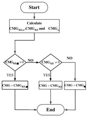
The algorithm of finding CMG is shown in Figure 4.

Figure 4. Finding Critical Machine Group (CMG) Algorithm

5.2. Corrected Kinetic Energy Function

Transient energy function after fault period is stored, nonetheless, all the transient kinetic energy is not turned into potential energy in the first swing of system separation [12-14]. Therefore, in various references such as reference[22-24], corrected kinetic energy is defined by Eq. (14) as follows:

𝐾𝐸𝐶𝑂₌1

2𝑀𝑒𝑞𝜔2 (14)

where, 𝑀𝑒𝑞 and 𝜔 are defined by Eq. (15,16):

𝑀𝑒𝑞=_𝑀𝑀_𝐶𝑀𝐺𝐶𝑀𝐺_+𝑀𝑀𝑁𝐶𝑀𝐺_{𝑁𝐶𝑀𝐺} (15)

𝜔 = 𝜔𝐶𝑀𝐺− 𝜔𝑁𝐶𝑀𝐺 (16)

𝜔𝑁𝐶𝑀𝐺and𝜔𝐶𝑀𝐺are defined by Eq. (17,18):

𝜔𝑁𝐶𝑀𝐺=∑ 𝑀𝑖𝜔𝑖 𝑀𝑁𝐶𝑀𝐺 𝑛𝑠𝑦𝑠 𝑖 (17) 𝜔𝐶𝑀𝐺=∑ _𝑀𝑀𝑖𝜔𝑖 𝐶𝑀𝐺 𝑛𝑐𝑟 𝑖 (18)

𝑀𝐶𝑀𝐺and𝑀𝑁𝐶𝑀𝐺are defined by Eq.(19,20):

𝑀𝐶𝑀𝐺= ∑𝑛𝑖=1𝐶𝑀𝐺𝑀𝑖 (19)

𝑀𝑁𝐶𝑀𝐺= ∑𝑛𝑖=1𝑁𝐶𝑀𝐺𝑀𝑖 (20) 5.3. Corrected Kinetic Energy Function

Start

End

4

It should be noted that since all of the transient kinetic energy is not turned into potential energy in the first swing of separation of system, critical kinetic energy that was obtained for each generator also does not affect fully in the first swing of system separation and like that kinetic energy should be corrected as follows in Eq. (21):

𝐾𝐸𝑐𝑟𝑖𝑡𝐶𝑂=1₂𝑀𝑒𝑞𝜔𝑐𝑟𝑖𝑡2 (21)

where,𝜔_{𝑐𝑟𝑖𝑡}is defined by Eq. 22:

𝜔𝑐𝑟𝑖𝑡= 𝜔𝑐𝑟𝑖𝑡𝐶𝑀𝐺− 𝜔𝑐𝑟𝑖𝑡𝑁𝐶𝑀𝐺 (22)

𝜔𝑐𝑟𝑖𝑡𝐶𝑀𝐺and 𝜔𝑐𝑟𝑖𝑡𝑁𝐶𝑀𝐺are defined by Eq. (23,24):

𝜔𝑐𝑟𝑖𝑡𝐶𝑀𝐺= ∑𝑛𝑖=1𝑐𝑟𝑀𝑖_𝑀𝜔_𝐶𝑀𝐺𝐶𝑅𝐼𝑇𝑖 (23)

𝜔𝑐𝑟𝑖𝑡𝑁𝐶𝑀𝐺= ∑𝑛𝑖=1𝑠𝑦𝑠𝑀_𝑀𝑖𝜔_{𝑁𝐶𝑀𝐺}𝐶𝑅𝐼𝑇𝑖 (24) 5.4. Stability Margin Index

After calculating the corrected kinetic energy and the critical kinetic energy for any disturbance and interval (Δt ) can be expressed index to determine the stability margin of the system as follows in Eq. (25):

𝑆𝑀𝐼 =_𝐾𝐸𝐾𝐸𝐶𝑂 𝑐𝑟𝑖𝑡𝐶𝑂 = 1 2𝑀𝑒𝑞𝜔2 1 2𝑀𝑒𝑞𝜔𝐶𝑟𝑖𝑡2 = ( 𝜔 𝜔𝐶𝑟𝑖𝑡) 2 (25)

The algorithm of Obtaining an index to determine the stability of the system for each interval (Δt ) is shown in Figure 5 . In Figure 5, when the index is closer to 1, the system is close to instability, and when this index is closer to zero, the system is more stable.

Figure 5. Achieving Stability Margin Index

6. Simulation and Results

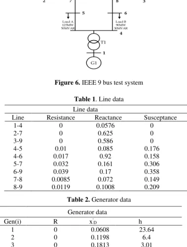
To test the proposed method, IEEE 9 Bus test system is used to provide a comparison between kinetic and critical kinetic energies of a single machine. The test system contains 3 generators and 9 buses, as shown in Figure 6.

Generator and line data are listed in Table 1 and Table 2, respectively. Two different cases are simulated and the applied three-phase fault is severe enough to become system

unstable and KE, δ, and ω for each generator and SF for the system are studied.

G2 G3 G1 T3 T2 T1 1 2 3 4 5 6 7 8 9 Load A 125MW 50MVAR Load B 90MW 30MVAR Load C 100MW 35MVAR

Figure 6. IEEE 9 bus test system

Table 1. Line data Line data

Line Resistance Reactance Susceptance

1-4 0 0.0576 0 2-7 0 0.625 0 3-9 0 0.586 0 4-5 0.01 0.085 0.176 4-6 0.017 0.92 0.158 5-7 0.032 0.161 0.306 6-9 0.039 0.17 0.358 7-8 8-9 0.0085 0.0119 0.072 0.1008 0.149 0.209

Table 2. Generator data

6.1. Case 1: (Fault Line 5-7 Near Bus5)

Since the synchronous reference frame is used, the speeds and angles are compared with the reference generator

(slack). δc and ωcrit are computed by employing the EAC

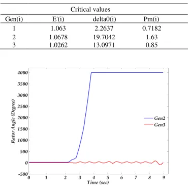
method and the previous equations; after the fault occurs at line 5-7 near bus 5 which is cleared after at 0.4 sec. Before transient stability assessment, load flow solution has been carried out to obtain initial values. These initial values are listed in Table 3 and Table 4. According to the Figures 7 and 8 can be found that the system will be unstable by this fault but did not specify the exact time of instability. With regards to Figure 9 that depicts SMI instability accurate time is clear. Figure 9 shows that the system is unstable before clearing fault means that the system has not the ability to absorb kinetic energy has been injected.

Table3. Results of load flow Load Flow

Gen(i) E'(i) delta0(i) Pm(i)

1 1.063 2.2637 0.7182

2 1.0678 19.7042 1.63

3 1.0262 13.0971 0.85

System is stable and Determine Stability Margin Index

End Start

Calculate Stability Margin Index (SMI) CO CO crit Calculate KE and KE 1 SMI YES System is Unstable IF NO Generator data Gen(i) R x' D h 1 0 0.0608 23.64 2 0 0.1198 6.4 3 0 0.1813 3.01

Table 4. Critical values

Figure 7. Rotor's angles when fault occurs in bus 5, clear after 0.4 sec

Figure 8. Rotor's speeds when fault occurs in bus 5, clear after 0.4 sec

Figure 9. SMI when the fault occurs in bus 5, clear after 0.4 sec.

6.2. Case2: (Fault at Line 6-8 Near Bus8)

In this case fault occurs at line 6-8 near bus 8 and clear

after 0.2 sec, we can see various δ and ω for each generator and SMI for the system. It can be realized According to figures 10, 11, and 12 the system is stable, but the stability margin and how much the system is close to instability cannot be found.

Figure 12. SMI when the fault occurs in bus 8, clear after 0.3 sec. Critical values

Gen(i) E'(i) delta0(i) Pm(i)

1 1.063 2.2637 0.7182

2 1.0678 19.7042 1.63

3 1.0262 13.0971 0.85

Figure 10. Rotor's angles when the fault occurs in bus 8, clear after 0.3 sec.

Figure 11. Rotor's speeds when the fault occurs in bus 8, clear after 0.3 sec

6

7. Conclusions

The proposed method is based on transient energy function methods, which can be used to determine transient stability directly without solving the power system equations numerically. It uses the energy conversion phenomena for any object. Due to problems in obtaining potential energy function, an index was introduced to determine the stability margin system used to kinetic energies term. The method uses the critical kinetic and kinetic energies which are compared with each other. If the critical kinetic energy is greater than the kinetic energy, then the system is considered unstable and if the kinetic energy is greater than the critical kinetic energy system is stable and determines the stability margin of the system. The proposed method is applied to the IEEE 9 Bus power system for several fault cases.

References

[1] C.-W. Liu, M.-C. Su, S.-S. Tsay, and Y.-J. Wang, "Application of a novel fuzzy neural network to real-time transient stability swings prediction based on synchronized phasor measurements," IEEE Transactions on Power Systems, vol. 14, pp. 685-692, 1999.

[2] R. Evans and C. Wagner, "Studies of transmission stability," Transactions of the American Institute of Electrical Engineers, vol. 45, pp. 51-94, 1926. [3] P. Kundur, N. J. Balu, and M. G. Lauby, Power system

stability and control vol. 7: McGraw-hill New York, 1994.

[4] V. Vittal and A. Bergen, "Power systems analysis,"

Prentice Hall, pp. 1-2, 1999.

[5] P. C. Magnusson, "The transient-energy method of calculating stability," Transactions of the American Institute of Electrical Engineers, vol. 66, pp. 747-755, 1947.

[6] H. Al Marhoon, I. Leevongwat, and P. Rastgoufard, "A practical method for power systems transient stability and security analysis," in PES T&D 2012, 2012, pp. 1-6.

[7] A. Michel, A. Fouad, and V. Vittal, "Power system transient stability using individual machine energy functions," IEEE Transactions on Circuits and Systems, vol. 30, pp. 266-276, 1983.

[8] Q. Jiang and Z. Huang, "An enhanced numerical discretization method for transient stability constrained optimal power flow," IEEE Transactions on Power Systems, vol. 25, pp. 1790-1797, 2010.

[9] C. Wang, K. Yuan, P. Li, B. Jiao, and G. Song, "A projective integration method for transient stability assessment of power systems with a high penetration of distributed generation," IEEE Transactions on Smart Grid, vol. 9, pp. 386-395, 2016.

[10] A. Priyadi, N. Yorino, O. A. Qudsi, and M. H. Purnomo, "CCT computation method based on critical trajectory using simultaneous equations for transient stability analysis," in 2014 6th International Conference on Information Technology and Electrical Engineering (ICITEE), 2014, pp. 1-6.

[11] M. Pavella, D. Ernst, and D. Ruiz-Vega, Transient stability of power systems: a unified approach to

assessment and control: Springer Science & Business Media, 2012.

[12] Y. Xue, T. Van Custem, and M. Ribbens-Pavella, "Extended equal area criterion justifications, generalizations, applications," IEEE Transactions on Power Systems, vol. 4, pp. 44-52, 1989.

[13] S. Mahdavi and A. Dimitrovski, "Coordinated voltage regulator control in systems with high-level penetration of distributed energy resources," in 2019 North American Power Symposium (NAPS), 2019, pp. 1-6.

[14] S. Mahdavi and A. Dimitrovski, "Integrated Coordination of Voltage Regulators with Distributed Cooperative Inverter Control in Systems with High Penetration of DGs," in 2020 IEEE Texas Power and Energy Conference (TPEC), 2020, pp. 1-6.

[15] N. Sarikhani and A. G. Mazidi, "Online Distribution System's Voltage Stability Margin Monitoring Using Neural Networks and Optimization Algorithm,"

Computational Research Progress in Applied Science & Engineering, vol. 2, pp. 23-27, 2016.

[16] H. P. S. Mahdavi, A. Dimitrovski and Q. Zhou, "Predictive and Cooperative Voltage Control with Probabilistic Load and Solar Generation Forecasting," in 2020 IEEE International Conference on Probabilistic Methods Applied to Power Systems (PMAPS), Liege, Belgium, 2020, pp. 1-6.

[17] H. Shokouhandeh, M. Ghaharpour, H. G. Lamouki, Y. R. Pashakolaei, F. Rahmani, and M. H. Imani, "Optimal Estimation of Capacity and Location of Wind, Solar and Fuel Cell Sources in Distribution Systems Considering Load Changes by Lightning Search Algorithm," in 2020 IEEE Texas Power and Energy Conference (TPEC), 2020, pp. 1-6.

[18] R. P. A. Taghavirashidizadeh, M. Hayerikhiyavi, M. Zahedi, "A Genetic Algorithm for Multi-Objective Reconfiguration of Balanced and Unbalanced Distribution Systrms in Fuzzy Framework," Journal of Critical Reviews, vol. 7(7), pp. 639-343, 2020. [19] F. Milano, "An open source power system analysis

toolbox," IEEE Transactions on Power systems, vol. 20, pp. 1199-1206, 2005.

[20] P. M. Anderson and A. Fouad, Power system stability: Wiley-IEEE Press, 2003.

[21] A. Pizano-Martianez, C. R. Fuerte-Esquivel, and D. Ruiz-Vega, "Global transient stability-constrained optimal power flow using an OMIB reference trajectory," IEEE Transactions on Power Systems, vol. 25, pp. 392-403, 2009.

[22] A. Vahidnia, G. Ledwich, E. Palmer, and A. Ghosh, "Dynamic equivalent state estimation for multi-area power systems with synchronized phasor measurement units," Electric power systems research, vol. 96, pp. 170-176, 2013.

[23] R. F. Gibson, E. O. Ayorinde, and Y.-F. Wen, "Vibrations of carbon nanotubes and their composites: a review," Composites science and technology, vol. 67, pp. 1-28, 2007.

[24] H. Richter, D. Simon, W. A. Smith, and S. Samorezov, "Dynamic modeling, parameter estimation and control of a leg prosthesis test robot," Applied Mathematical Modelling, vol. 39, pp. 559-573, 2015.