Delay range dependent Robust Stability for Uncertain Singular Systems with Interval Time varying Delays

Delay-range-dependent Robust Stability for Uncertain

Singular Systems with Interval Time-varying Delays

Pin-Lin Liu

Department of Automation Engineering Institute of Mechatronoptic System, Chienkuo Technology University, Changhua, 500, Taiwan, Republic of China

*Corresponding Author: lpl@cc.ctu.edu.tw

Copyright © 2013 Horizon Research Publishing All rights reserved.

Abstract

In this paper, we consider the delay-range- dependent robust stability problem of uncertain singular system with interval time-varying delays. Stability criteria, which guarantee the concerned singular system is regular, free and stable, is derived in terms of linear matrix inequalities (LMIs) by introducing some identical equations with integral inequality approach (IIA) and using the Leibniz-Newton formula to reduce the conservatism of the results. The upper bound of time-delay can be obtained by using the modified generalized eigenvalue minimization problem (GEVP) technique such that the system can be stabilized for all time-delays. Finally, numerical examples show the method presented in our paper is more effective and less conservative than the existing ones.

Keywords

Singular Time Delay Systems, Integral Inequality Approach (IIA), Delay- Dependence, Linear Matrix Inequality (LMI)

1. Introduction

Engineering processes often involve both nonlinear and time-delay models. In many physical and biological phenomena, the rate of variation in the system state depends on past states. Time delay phenomena were first discovered in biological systems and were later found in many engineering systems, such as mechanical transmissions, fluid transmissions, metallurgical processes, and networked control systems. They are often a source of instability and poor control performance. Therefore, many efforts have been made for the stability problems for various delayed systems [1-2, 4-14, 16-31]. Moreover, because of unavoidable factors, such as modeling error, external perturbation and parameter fluctuation, the time delay systems certainly involve uncertainties such as perturbations and component variations, which will change the stability of time delay systems. And in recent years, the stability analysis issues for time delay systems in the presence of parameter uncertainties perturbations have

stirred some initial research attention [4, 5, 8, 12, 16, 19, 20, 22-25, 31].

Singular systems have found numerous practical applications: e.g., engineering systems, social systems, economic systems, biological systems. Unlike classical state space representation via a set of ordinary differential equations, singular system can be viewed as a composite formed by several interconnected systems with two layers: dynamic property described by differential equation and interconnection property expressed by algebraic equation. Therefore, some results on the stability of singular systems are achieved [1, 5-8, 12-13, 16-18, 20-25, 27-30] and the references therein. The existing stability criteria for singular time-delay systems can be classified into two types: delay- independent [5, 24, 25, 30] and delay-dependent [1, 6-8, 12-13, 16-19, 21-23, 26, 28-29, 31]. Generally, delay- dependent conditions are less conservative than the delay- independent ones, especially when the time delay is small. For singular systems with delays, several kinds of simple Lyapunov–Krasovskii functionals, i.e. functionals parameterized with constant matrices, have been proposed, which lead to different levels of conservatism due to the different model transformations and the bounding techniques for some cross-terms [7, 8]. A tighter bounding for cross-terms can reduce the conservatism. However, there are no obvious ways to obtain less conservative results, even if one is willing to expend more computational effort on the problem, and to find a tighter bound for the cross-terms. This is the serious limitation for these criteria. To overcome this limitation, one has to find some more general Lyapunov-Krasovskii functional (LKF) for handling the delay-range-dependent robust stability problem for singular systems. To the best of our knowledge, this delay- range-dependent robust stability problem has not been fully investigated for singular systems with time-varying delay, which motivates the present study.

the stability criteria for time-varying delay systems in [17, 18, 20, 27] are conservative because they do not take into account the information of the lower bound of delay. To the best of authors’ knowledge, there have been few results on the delay-range-dependent robust stability of the singular systems with time-varying interval delays, which remain as an interesting research topic.

Motivated by the above discussions, we propose the improved delay-range-dependent robust stability for singular systems with time-varying interval delay and uncertainties. First, by defining a novel Lyapunov function, a delay-range-dependent stability criterion for the nominal singular time- delay system is established in terms of LMIs. Next, less conservative result is obtained by considering some useful terms when estimating the upper bound of the derivative of Lyapunov functional and introducing the additional terms into the proposed Lyapunov functional, which includes the information of the range. The maximum allowable value of the time delay can be obtained by solving a set of linear matrix inequalities (LMIs) and the modified generalized eigenvalue minimization problem (GEVP) algorithm. Finally, Numerical examples demonstrate that the results obtained in this paper are effective and are a significant improvement over previous ones.

2. Stability Description and

Preliminaries

Consider the following uncertain singular system with an interval time-varying delay as follows:

( ) ( ( )) ( ) ( ( )) ( ( )),

Ex t = A+ ∆A t x t + B+ ∆B t x t h t− t >0, (1a) with the initial condition

2 ( ) ( ), [ ,0],

x t =φ t t∈ −h (1b) where ( )_{x t} n

R

∈ is the state vector of the system;

, n n

A B R_∈ × _{are constant matrices; The matrix E R∈} n n× maybe singular, without loss generality, we suppose

;

rankE r n= ≤

φ

(

t

)

is a continuously real-valued initial function on [−h2,0]. ( )h t is a time-varying delay which satisfies:

1 h t( ) 2,

h ≤ ≤h h t( )≤hd<1, ∀ ≥t 0, (2)

where h1and h2 are the lower and upper delay bounds, respectively, h h1, 2 and hd are constants and 0≤h h1< 2. Time-varying parametric uncertainties ∆A t( ) and ∆B t( ) are assumed to be of the following form:

[

∆A t( ) ∆B t( )

]

=MF t N N( )

[

a b

]

, (3)

where M N, a,andNbare known real constant matrices

with appropriate dimensions, and ( )F t is an unknown, real, and possibly time-varying matrix with Lebesgue- measurable elements satisfying

( ) ( ) , .

T _{t F t I t}

F ≤ ∀ (4)

The main objective is to find the range of h1≤h t( )≤h2 and guarantee stability for the uncertain singular time-varying delay systems (1). Here, definitions fundamental lemmas are reviewed.

Definition 1 [3]: The pair ( , )E A is said to be regular if det(sE A− )is not identically zero.

Definition 2[3]: The pair ( , )E A is said to be impulse free if deg(det(sE A− )) rank .= E

Definition 3[3]:For a given scalar h>0, the singular time-varying delay system (1) is said to be regular and impulse free for any constant time delay

h

satisfying

0≤ ≤h h,it the pairs ( , )E A and ( ,E A B+ ) are regular and impulse free.

Remark 1:The regularity and the absence of impulses of the pair ( , )E A ensures the system (1) with time delay h≠0 to be regular and impulse free, while the fact that the pair

( ,E A B+ ) is regular and impulse free ensures the system (1) with time delay h=0 to be regular and impulse free.

Lemma 1 [15]: The singular system Ex t( )= Ax t( )is regular, impulse free, and stable, if and only if there exists a matrix

Psuch that:

0,

T_{P PA}

A + < (5a) with the following constraint

0

T_E T_P

P =E ≥ . (5b)

Lemma 2 [17]: For any positive semi-definite matrices: 11 12 13

12 22 23 13 23 33

0,

T

T T

X X X

X X X X

X X X

 

 

=_{ }≥

 

 

(6a)

the following integral inequality holds

33 ( )

( )

11 12 13 12 22 23 13 23

( ) ( )

( ) ( ( )) ( )

( )

( ( )) .

0 ( )

t T

t h t

t T T T

t h t

T

T T

s x s ds

x X

t t h t s

x x x

x t

X X X

x t h t ds

X X X

x s

X X

− − −∫

≤∫  − ×

   

   ₋ 

   

   

   

 





(6b)

Lemma 3[2]. The following matrix inequality: ( ) ( )

0, ( ) ( )

T

Q x S x

x R x

S

 

<

 

  (7a)

where ( )_{Q x Q}T( ), ( )_{x R x} T( ) and ( )_{x S x} R

= = depend affine

on

x

,

is equivalent to

( ) 0,

R x < (7b) ( ) 0,

and

1

( ) ( ) ( ) ( ) 0.T

Q x S x₋ R− xS x _{< (7d)}

Lemma 4[2]. Given matrices _Q=QT, , ,_{D E and}

0

T

R R= > of appropriate dimensions, ( ) T T( ) T 0,

Q DF t E+ +E F t D < (8a)

for all ( )F t satisfying T( ) ( )_{t F t I},

F ≤ if and only if there exists some ε >0 such that

1 _0.

T T

Q₊εDD ₊ε−E E_{< (8b)} In this paper, a new Lyapunov functional is constructed, which contains the information of the lower bound of delay

1

h and upper bound_h2.

The nominal unforced time delay singular system (1) can be written as follows:

( ) ( ) ( ( )).

Ex t =Ax t +Bx t h t− (9) The following Theorem 1 presents a delay-range- dependent result in terms of LMIs and expresses the relationships between the terms of the Leibniz–Newton formula.

Theorem 1: For three given positive scalars

h h

1

, ,

2 and

,

d

h

the time-delay singular system (9) is asymptotically stable if there exist matrices T 0, T 0,

i i

P=P > Q Q= > 0( 1,2,3; 1,2),

T

j j i j

R =R > = = S with appropriate

dimensions, positive semi-definite matrices: 11 12 13

12 22 23 13 23 33

0,

T

T T

X X X

X X X X

X X X

    =_{ }≥     and

11 12 13 12 22 23 13 23 33

0

T

T T

Y Y Y

Y Y Y Y

Y Y Y

 

 

=_{ }≥

 

 

such that the following LMIs hold:

11 12 15 16

12 22 23 24 25 26 23 33

24 44

15 25 55

16 26 66

0 0

0 0 0 0

0,

0 0 0 0

0 0 0

0 0 0

T

T

T

T T

T T

Ξ Ξ Ξ Ξ 

 

Ξ Ξ Ξ Ξ Ξ Ξ

 

 _{Ξ Ξ} 

Ξ = <

Ξ Ξ

 

_{Ξ Ξ Ξ} 

 

Ξ Ξ Ξ 

 

(10a)

1 33

( ) 0,

T _E

E R X− ≥ (10b)

2 33

( ) 0,

T _E

E R Y− ≥ (10c)

with the following constraint

0.

T_E T_P

P =E ≥ (10d) where _{Z R∈} n n r× −( ) _{is any matrix with full column rank and} satisfies_ET_{Z =}0_and

11 1 2 3

11 13 13 2

12 2 12 13 23

15 2 1 16 21 2

( ) ,

( ) ,

, ,

T

T T T

T T

T T T

T T

P PA ZS S A Q Q Q

A A Z

E h

E X X X

PB S BZ E h X X X E

h A R h A R

= + + + + + + Ξ + + + = + + − + Ξ = = Ξ Ξ

22 3 21 11 13 13 2 22 23 23

22 23 23 11 13 13

21 21

23 21 12 13 23

24 21 12 13 23 21 12 13 23

25 2 1 26 21 2

33 1 21 11 13 13

(1 ) (

) ,

( ) ,

( ) ,

, ,

( )

T T T

d

T T

T T T

T T T

T T

T T

Q

h E h X X X h X X X

E

h Y Y Y h Y Y Y

E h

E Y Y Y

E

h h

E X X X Y Y Y

h B R h B R

E

Q E h Y Y Y

= − − + + + + − − Ξ + − − + + + = − + Ξ = − + + − + Ξ = = Ξ Ξ =− + + + Ξ

44 2 21 22 23 23 21 22 23 23

55 2 1 66 21 2

,

( ) ,

, .

T T T _E

Q E h Y Y Y h X X X

h R h R

=− + − − + − −

Ξ

= − = −

Ξ Ξ

Proof: Consider the time-varying delay singular system (9), using the Lyapunov- Krasovskii functional candidate in the following form, we can write:

1 2 2 1 2 1 2 0 1 3 ( ) 2 ( ) ( ) ( ) ( ) ( ) ( ) ( ) ( ) ( ) ( ) ( )

( ) ( ) (11)

t t

T T T

t th th

t T t T T

t h t h t

t

h T T

t h

V x x t PEx t x s x s dsQ x sQx s ds

sQx s ds s Ex s dsd

x x E R

s Ex s dsd

x E R

θ θ θ θ − − − − + − − + = +∫ +∫ +_∫ +_{∫ ∫} +∫ ∫    

Calculating the derivative of (11) with respect to t>0

along the trajectories of (9) leads to

1 2 3

1 1 1 2 2 2

1 2 3 2 21 1 ( ) ( )( ) ( ) ( ) ( ( )) ( ( )) ( ) ( )( ) ( ) ( ) ( ) ( ) ( )

( ( ))(1 ( )) ( ( )) ( ) ( )

( ) ( ) ( ) (

T T T

t

T T T

T T

T T T

T T T T

V x x t PA A P x t x t PBx t h t

t h t Px t t Q Q Q x t

x B x

t Qx t t Qx t

x h h x h h

t h t h t Qx t h t t Ex t

x x h E R

t Ex t s REx

x h E R x E

= + + − + − + + + − − − − − − − − − − + − +   _{ }  

 2

1

2 2

1 2 3

1 1 1 2 2 2

3 1 2 2 21 ) ( ) ( ) ( )( ) ( ) ( ) ( ( )) ( ( )) ( ) ( ) ( ) ( ) ( )

( ( ))(1 ) ( ( ))

( ) ( ) ( )

t t h

t h T T

t h

T T

T

T T T

T T

d

T T T T

s ds

s REx s ds

x E

t PA P Q

x A

x t t PBx t h t

Q Q x

t h t Px t t Qx t

x B x h h

t Q x t

x h h

t h t h Qx t h t

x

t Ex t t Ex

x h E R x h E R

− − − ∫ −∫ ≤ + + + + + − + − − − − − − − − − − − + +       2 1 2 1 2

1 2 3

1 1 1 2 2 2

3 1 2 21 ( ) ( ) ( ) ( ) ( ) = ( )( ) ( ) ( ) ( ( )) ( ( )) ( ) ( ) ( ) ( ) ( )

( ( ))(1 ) ( ( ))

( ) (

t T T

t h

t h T T

t h T T T T T T T T d T T t

s Ex s ds

x E R

s Ex s ds

x E R

t PA P Q Q Q x t

x A

t PBx t h t x

t h t Px t

x B

t h Qx t h

x

t Q x t

x h h

t h t Qx t h t

x h

t

x E h R

− − − −∫ −∫ + + + + + − + − − − − − − − − − − − + +      2 1 2 2 1 2 2 1 33 2 33 33 33 ) ( ) ( ) ( ) ( ) ( ) ( ) ( ) ( ) ( )

( ) ( ) (12)

t _{T T}

t h

t h T T

t h

t T T

t h

t h T T

t h

Ex t h R

s Ex s ds

x E R X

s Ex s ds

x E R Y

s Ex s ds

x E X

s Ex s ds

x E Y

− − − − − − −_∫ − −∫ − −∫ −∫         

2

2

33 ( )

33 ( ) 33

( )

( )

( )

( )

( )

( ) , (13)

t T T

t h

t h t T T t T T

th t h t

s

Ex s ds

x

E X

s

Ex s ds

s

Ex s ds

x

E X

x

E X

− − − −

−∫

= −

_∫

−

_∫













and 1 2 1 2 33 ( )

33 _{( )} 33

( )

( )

( )

( )

( )

( ) ,

t h T T

t h

t t T T t h T T

th t h t

s

Ex s ds

x E Y

s

Ex s ds

s

Ex s ds

x

E Y

x

E Y

− − − − − −

−∫

= −

_∫

−

_∫













(14) Using the Leibniz-Newton formula

( ) ( ) t ( ) ,

t h

x t x t h− − = ∫− x s ds and Lemma 2, we obtain:

33 ( )

( )

11 12 13 12 22 23 13 23

11 12

2 2

13 ( ) 12

( )

( )

( )

(

( ))

( )

( )

(

( ))

0

( )

( )

( )

( )

(

( ))

( )

( )

(

( ))

t T

t h t

t T T T

t h t

T

T T

T T

t T

t h t T

s

x s ds

x

X

t

t h t

s

x

x

x

x t

X

X

X

x t h t ds

X

X

X

x s

X

X

t

x t

t

x t h t

x h

X

x h

X

t

x s ds

x

X

t h t

x

− − −

−∫

≤

∫



_

−



_

×



 





 

₋





 





 





 



≤

+

−

+

∫

+

−











22 2

23 ( )

13 23

( ) ( )

11 13 13 2

12 13 23 2

12 13 23 2

( )

(

( ))

(

( ))

(

( ))

( )

( )

( )

( )

(

( ))

( )(

) ( )

( )(

) (

( ))

(

( ))(

T T t T

t h t

t T T t T T

t h t t h t

T T

T T

T T T

x t

hX

t h t

x t h t

x

h X

t h t

x s ds

x

X

s ds x t

s ds x t h t

x

X

x

X

t

x t

x

h X

X

X

t

x t h t

x

h X

X

X

t h t

x

h X

X

X

− − −

+

−

−

+

−

∫

+

∫

+

∫

−

=

+

+

+

−

+

−

+

−

−

+







22 23 23 2

) ( )

(

( ))(

) (

( ))

T T

x t

t h t

x t h t

x

h X

X

X

+

−

−

−

−

(15) Similarly, we have

2

( )

33

11 13 13 21

12 13 23

21 2

12 13 23 2 21

22 23 23

2 21 2

( )

( )

(

( ))(

) (

( ))

(

( ))(

) (

)

(

)(

) (

( ))

(

)(

) (

)

t h t T t h

T T

T T

T T T

T T

s

x s ds

x

X

t h t

x t h t

x

h X

X

X

t h t

x t

x

h

X

X

X

h

t

x t h t

x

h h X

X

X

t

x t

x

h h

X

X X

h

− −

−∫

≤

−

+

+

−

+

−

−

+

−

+

−

−

+

−

+

−

−

−





(16) 1 33 ( )

11 13 13

1 21 1

12 13 23 1 21

12 13 23

21 1

22 23 23 21

-

( )

( )

(

)[

] (

)

(

)[

] (

( ))

(

( ))[

] (

)

(

( ))[

] (

( ))

t h T

t h t

T T

T T

T T T

T T

s

x s ds

x

Y

t

x t

x

h h

Y

Y

Y

h

t

x t h t

x

h h Y

Y

Y

t h t

x t

x

h

Y

Y

Y

h

t h t

x t h t

x

h Y

Y

Y

− −

∫

≤

−

+

+

−

+

−

−

+

−

+

−

−

+

−

+

−

−

−

−





(17) and 2 ( ) 33

11 13 13 21

12 13 23

21 2

12 13 23 2 21

22 23 23

2 21 2

-

( )

( )

(

( ))[

] (

( ))

(

( ))[

] (

)

(

)[

] (

( ))

(

)[

] (

)

(18)

t h t T t h

T T

T T

T T T

T T

s

x s ds

x

Y

t h t

x t h t

x

h Y Y Y

t h t

x t

x

h

Y Y Y

h

t

x t h t

x

h h Y Y Y

t

x t

x

h h

Y

Y

Y

h

− −

∫

−

+

+

−

≤

+

−

−

+

−

+

−

−

+

−

+

−

−

−

−





With the operator for the term xT( ) (t ET h2R1+h21R2) ( )Ex t as follows: 1 2 2 21 1 2 2 21 1 2 2 21 1 2 2 21 1 2 2 21 1 2 2 21

( ) (

) ( )

[ ( )

(

( ))] (

)[ ( )

(

( ))]

( )

(

) ( )

( )

(

) (

( ))

(

( ))

(

) ( )

(

( ))

(

) (

( ))

T T T T T T T T T T T

t

Ex t

x

E

h

R

h

R

x t Bx t h t

h

R

h

R

x t Bx t h t

t h

Ax t

x

A

h

R

h

R

t h

Bx t h t

x

A

h

R

h

R

t h t h

Ax t

x

B

h

R

h

R

t h t h

Ax t h t

x

B

h

R

h

R

+

=

+

−

+

+

−

=

+

+

+

−

+

−

+

+

−

+

−





(19)

To obtain an easily solvable LMI, we introduce the matrix

( )

n n r

Z R

_∈

× −

satisfying _ET_{Z =}0_{and rank Z n r= − [18, 19,}

22].Then, we have

0 2 ( )

T

_{t Z x t}

T T

( )

x

E

S

=

_

(20) Substituting the above equations (13)-(20) into (12) yields

2 1 2 1 33 2 33

( )

( ) ( )

( ) (

) ( )

( ) (

) ( ) (21)

t

T T T

t _{t h}

t h T T

t h

V

x

t

t

x E R X

s

Ex s ds

s

Ex s ds

x E R Y

ξ

ξ

−

− −

≤

Ω

−

_∫

−

−

_∫

−



_

_





where

( )

( )

(

( ))

(

1

)

(

2

)

T

_t

_x

T

_t

_x

T

_{t h t}

_x

T

_t

_{h x}

T

_t

_h

ξ

=



_

−

−

−



_

and

11 12

12 22 23 24

23 33 24 44 0 0 , 0 0 0 0 T T T

Ω Ω 

_{Ω Ω Ω Ω} 

 

Ω =

 _{Ω Ω} 

 

Ω Ω

 

where

11 1 2 3

11 13 13 1 2

2 2 21

12 2 12 13 23

1 2

2 21

22 3 21 11 13 13 2 22 23 23 11 13 13 22 23 23

21 21

(

)

(

) ,

(

)

(

) ,

(1

)

(

)

(

T

T T T

T T T

T T T

T

T T T

d

T T T

P PA

Z

S

S A Q Q Q

A

A

Z

E

A

h

h

h

E

X

X

X

A

R

R

PB S B

Z

E

h

X

X

X

E

B

h

h

A

R

R

Q

h

E

h

X

X

X

h

X

X

X

E

h

Y Y

Y

h

Y

Y

Y

B

=

+

+

+

+ +

+

Ω

+

+

+

+

+

=

+

+

−

+

Ω

+

+

= − −

+

+

+

+

−

−

Ω

+

+

+

+

−

−

+

_{2 1 21 2}

23 21 12 13 23

24 21 12 13 23 21 12 13 23 33 1 21 11 13 13

44 2 21 22 23 23 21 22 23 23

) ,

(

) ,

(

) ,

(

) ,

(

) .

T T T

T T T

T T

T T T

B

h

R

h

R

E

h

E

Y

Y

Y

E

h

h

E

X

X

X

Y

Y

Y

E

Q

E

h

Y Y

Y

E

Q

E

h

Y

Y

Y

h

X

X

X

+

=

−

+

Ω

=

−

+

+

−

+

Ω

=

−

+

+

+

Ω

=

−

+

−

−

+

−

−

Ω

complement of Lemma 2 we can get Ω <0, 1 33

( ) 0,

T _E

E R X− ≥ E R YT( 2− 33) 0≥ for any ( ) 0.ξ t ≠ Therefore, the interval time-varying delay system (9) is asymptotically stable if (10) is true. Thus, the proof is complete.

3. Robust for Uncertain Singular

Interval Time-varying Delay System

In the section, extending Theorem 1 to uncertain singular system (1) with interval time-varying delays yields the following Theorem 2.

Theorem 2: For three given positive scalars h h1, ,2 and ,

d

h the uncertain singular time-varying delay system (1) is asymptotically stable if there exist symmetry positive-definite matrices _{P P=} T_>0, T _0,

i i

Q Q= >

0

T

j j

R

=

R

>

( 1,2,3;i= j=1,2) ε >0, S with appropriate dimensions, positive semi-definite matrices

11 12 13 12 22 23 13 23 33

0,

T

T T

X

X

X

X

X

X

X

X

X

X









=

_

_

≥









and

11 12 13

12 22 23

13 23 33

0

T

T T

Y

Y

Y

Y

Y

Y

Y

Y

Y

Y

 

 

 

 

 

=

≥

such that the following

LMIs hold:

15 16

11 12

23 24 25 26

12 22

23 33

24 44

15 25 55 2 1

16 26 66 21 2

66 2 1 21 2

0 0

0

0

0

0

0

0

0,

0

0

0

0

0

0 0

0

0 0

0

0 0 0

T T T T T T T

T T

PM

M

h R

M

h R

I

h

M R

h

M R

ε













































Ξ

Ξ

Ξ Ξ

Ξ Ξ

Ξ

Ξ

Ξ Ξ

Ξ Ξ

Ξ =

Ξ

Ξ

<

Ξ Ξ

Ξ

Ξ Ξ

Ξ

−

Ξ

(22a)

1 33

(

)

0,

T

_E

E R X

−

≥

(22b)

2 33

(

)

0,

T

_E

E R Y

−

≥

(22c)

with the following constraint

0.

T_E T_P

P =E ≥ (22d) where

11 12 22

11

,

12

,

22

,

T T T

a a a b b b

N N

N N

N N

ε

ε

ε

= +

Ξ

=

Ξ

+

=

Ξ

+

Ξ

Ξ

Ξ

,( , 1,2,...,6; 6)

ij i j= i j< ≤

Ξ are defined in (10).

It is, incidentally, worth noting that the singular uncertain time-varying delay system (1) is asymptotically stable, that

is, the uncertain parts of the nominal system can be tolerated within allowable time delay

h

1

≤

h t

( )

≤

h

2

.

Proof: Replacing A and B in (10) with A MF t N+ ( ) a

and B MF t N+ ( ) ,b respectively, we apply Lemma 4 [2] for

system (1) is equivalent to the following condition:

( )

T

( ) <0,

T

d

F t

e e

F t

d

Ξ +

Γ

Γ Γ

+

Γ

(23) where Γd=

[

PM 0 0 0 h2R1M h21R2M

]

and

[

0 0 0 0 .

]

e= Na Nb

Γ

By lemma 4 [2], a sufficient condition guaranteeing (10) for system (1) is that there exists a positive number ε >0 such that

1 T T

_0.

d d

ε

e e

ε

−

Ξ +

Γ Γ

+

Γ Γ

<

(24) Applying the Schur complement shows that (24) is equivalent to (22a). This completes the proof.

When h1=0, Theorem 1 reduces to the following Corollary 1.

Corollary 1: For a give scalarh>0,hd>0, the time-delay

singular system (9) is asymptotically stable if there exist symmetric positive-definite matrices _{P P=} T_>0,

0,

T

Q= > Q _{R R=} T_>0, _{and matrix S of appropriate}

dimensions and a positive semi-definite matrix

11 12 13 12 22 23 13 23 33

0

T

T T

X

X

X

X

_X

_X

_X

X

X

X









=

_

_

≥









such that the following LMIs

hold:

0,

T_E T_P

P =E ≥ (25a) 11 12 13

12 22 23 13 23 33

0,

T

T T

Ψ Ψ Ψ 

 

Ψ =_Ψ Ψ Ψ _<

_{Ψ Ψ Ψ} 

  (25b)

and

33

(

) 0, (25c)

T

_R

_E

E

−

X

≥

where

Z R

∈

n n r× −( ) is any matrix satisfying T_Z 0

E =

and

11

11 13 13

12 1 12 13 23

13 22 22 23 23

23 33

(

) ,

(

) ,

,

(1

)

(

) ,

,

.

T

T T T

T T

T T T

T T T

d T

P PA PA

Z

S

S A Q

A

A

Z

h

E

E

X

X

X

P

_A

S B

_Z

_E

h

_X

_X

_X

E

h R

A

h

Q

E

hX

X

X

E

h R

B

hR

=

+

+

+

+

+

Ψ

+

+

+

=

+

+

−

+

Ψ

=

= − −

+

−

−

Ψ

Ψ

=

= −

Ψ

Ψ

Proof: Consider the singular time-varying delay system (9), using the Lyapunov- Krasovskii functional candidate in the following form, we can rewrite as

( ) 0

( )

( )

( )

( ) ( )

( )

( )

(26)

t

T T

t _{t h t}

t _{T T}

h t

V

x

x

t PEx t

x

s Qx s ds

s REx s dsd

x

E

θ

θ

−

− +

=

_{+ ∫}

+∫ ∫

_



Similar to the above analysis, one can get that V x( ) 0t <

holds if Ψ <0.Thus, the proof is completed.

Now, extending Corollary 1 to time delay singular uncertain system (1) with time-varying structured uncertainties yields the following Corollary2.

Corollary 2: For given scalar h>0,hd>0, the

time-delay singular system (1) is asymptotically stable if there exist symmetric positive-definite matrices_{P P=} T_>0,

0,

T

Q= > Q _{R R=} T_>0,

_ε

_>0, _{and matrix S of}

appropriate dimensions and a positive semi-definite matrix

11 12 13 12 22 23 13 23 33

0

T

T T

X X X

X X X X

X X X

 

 

 

 

 

= ≥ such that the following LMIs

hold:

0,

T_E T_P

P =E ≥ (27a)

11 12 13

12 22 23

13 23 33

0

₀

0

T T

a a a b

T T

T

b a b b

T T

T T

PM

N N

N N

N N

N N

hRM

P

h

R

I

M

M

ε

ε

ε

ε

ε

 

 

 

 

 

 

 

+

+

Ψ

Ψ

Ψ

+

+

Ψ

Ψ

Ψ

Ψ =

<

Ψ

Ψ

Ψ

−

(27b) and

33

( ) 0, (27c)

T _{R E}

E −X ≥

where Z follows the same definition as that in Theorem 1, and

Ψ

ij

( , 1,2,3;

i j

=

i j

< ≤

3)

are defined in (25).

Remark 1: It is interesting to note that h h1, ,2 appear linearly in (10a) and (22a). Thus a generalized eigenvalue problem as defined in [2] can be formulated to solve the minimum acceptable 1/h2 (or 1/h1 ) and therefore the maximum h2(orh1) to maintain robust stability as judged by these conditions.

In this way, our optimization problem becomes a standard generalized eigrnvalue problem, then which can be solved using GEVP technique. From this discussion, we have the following Remark 2.

Remark 2: Theorem 2 provides delay-dependent asymptotic stability criteria for the time-varying delay singular systems (1) in terms of solvability of LMIs [2]. Based on them, we can obtain the maximum allowable delay bound (MADB) h1≤h t( )≤h2, such that (1) is stable by solving the following convex optimization problem:

2

Maximize

Subject to Theorem 2

h

 

 (28)

Inequality (28) is a convex optimization problem and can be obtained efficiently using the MATLAB LMI Toolbox.

To show usefulness of our result, let us consider the following numerical examples.

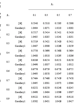
Table 1. MADBs h2with givenh1 for different hd in example 1

d

h

1

h 0.1 0.3 0.5 0.7

0.1 [16] 0.5348 0.5318 0.5305 0.5300

Corollary1 1.0484 1.0271 1.0213 1.0202

0.2 [16] 0.5517 0.5414 0.5411 0.5410

Corollary1 1.0485 1.0285 1.0241 1.0231

0.3 [16] 0.5519 0.5421 0.5420 0.5411

Corollary1 1.0487 1.0300 1.0268 1.0259

0.4 [16] 0.5750 0.5690 0.5688 0.5684

Corollary1 1.0488 1.0318 1.0295 1.0286

0.5 [16] 0.6186 0.6154 0.6151 0.6150

Corollary1 1.0490 1.0337 1.0321 1.0312

0.6 [16] 0.6776 0.6759 0.6758 0.6755

Corollary1 1.0493 1.0358 1.0347 1.0338

0.7 [16] 0.7464 0.7460 0.7459 0.7458

Corollary1 1.0495 1.0381 1.0372 1.0364

0.8 [16] 0.8252 0.8250 0.8248 0.8245

Corollary1 1.0498 1.0404 1.0396 1.0387

0.9 [16] 0.9122 0.9121 0.9120 0.9118

Corollary1 1.0502 1.0431 1.0426 1.0417

4. Illustrative Examples

Example 1: Consider the following time delay singular systems:

( ) ( ) ( ( ))

Ex t =Ax t +Bx t h t− (29)

where 1 0 , 0.5 0 , 1.1 1 .

0 0 0 1 0 0.5

E=_{ } A=_ _ B=_− _

−

     

Find the delay-range 0≤h1≤h t( )≤h2 to guarantee the above system (29) to be asymptotically stable.

Solution: Choosing _{0 0} 1 0 Z_{= } _

 

and taking the parameters

1 0.1

[image:6.595.296.547.190.540.2]

for any delay time _{[ , ] [0.1,1.0641].h h1 2 ∈} Comparison with other results is illustrated in Table 1. From Table 1, one can see that our results for this example give larger upper bounds of time-delay than the ones in [16]. By setting

1 0

h = and different hd the upper bounds on the time delay

from Corollary 1 are shown in Table 2, in which “-” means that the results are not applicable to the corresponding cases. For comparison, the Table 2 also lists the upper bounds obtained from the criteria in [1, 6-8, 17, 19, 20, 22, 23, 26, 28, 29, 31]. It can be seen that our methods are less conservative. The simulation of the system (26) for h=1.06 is depicted in Fig.1 with the initial state

[

−1 1 .

]

T

Table 2. MADBs h2for various hd in example 1

Methods hd

[image:7.595.59.295.271.724.2] [image:7.595.314.546.342.571.2] [image:7.595.338.523.621.728.2]

0 0.3 0.75

[1, 28] - - -

[29] 0.5567 - -

[8] 0.8707 - -

[6] 0.9091 - -

[7] 0.9689 - -

[26] 1.0423 - -

[17, 19, 22, 23,

31] 1.0660 - -

[20] 1.0660 1.0130 0.6496

Corollary 1 1.0660 1.0263 1.0164

Figure 1. The simulation of the example 1 forh=1.06 sec

Example 2: For convenience of comparison, consider the

following time-delay system [4, 6, 7, 21].

( ) ( ) ( ( ))

Ex t =Ax t +Bx t h t− (30)

where 1 1 , 1 0 , 1 1 .

1 1 0 1 1 1

E=_− _ A=_− _ B=_ − _

− − −

     

Solution: In this example, we choose

[

0 1 .

]

T

Z= For

1 0

h = and hd=0 the system (30), we are able to find a feasible solution for the set of LMIs for any

1 2

[ , ] [0,1.1547].h h ∈ This means that the maximum allowable delay bound (MADB) under which the system is uniformly asymptotically stable is 1.1547. Table 3 lists the maximum allowable delay bound (MADB) as judged by the criteria in [4, 6, 7, 21]. We can see from this table that there is still room for reducing the conservativeness by comparing with the numerical solution, but we know that with fewer matrix variables the stability results obtained in Corollary 1 is less conservative than the one in [4, 6, 7] and the same as [21]. Using these data, a simulation program has been written in Matlab. As Fig. 2 shows, the simulation of the above system (30) for h2=1.1547 with the initial state

[

1 1 .

]

T

−

Figure 2. The simulation of the example 2 forh=1.1547 sec Table 3. Comparison of MADBs h2in example 2 for different methods

and number of variables

Methods h2 Number of _variables

[6] <1 4

[7] 1.150 9

[4] 1.1547 7

[21] 1.1547 5

Corollary 1 1.1547 5

( ) ( ( )) ( ) ( ( )) ( ( )),

Ex t = A+ ∆A t x t + B+ ∆B t x t h t− (31) where

1.0 0 _, 0.4 0.2 _, 1 1.0 _,

0 0 0 1.0 0 0.3

0.1 0 _, 0.05 0 _, 0.05 0 _.

0 0.1 a 0 0.05 b 0 0.05

E A B

M N N

−

     

=_{ } =_{ } =_{ }

−

     

−

     

=_{ } =_{ } =_{ }

−

     

Solution: Choosing

Z

= 



0 0

_{1 0}









and taking the various

parameters ,hd the computed maximum upper bounds of

2,

h which guarantee the system (31) is regular, impulse free and robustly asymptotically stable for given bounds of h1, are listed in Table 4. Table 4 indicates that the time delay h2 decreases when the hd increases. We claim that the

sharpness of the upper bound delay timeh2 is negatively correlated with .hd For h1=0 and hd=0 the system (31),

we are able to find a feasible solution for the set of LMIs for any [ , ] [0,1.1782].h h1 2 ∈ This means that the maximum allowable delay bound (MADB) under which the system is uniformly asymptotically stable is 1.1782.Fig. 3 shows, the simulation of the above system (31) for h2=1.17 with the initial state

[

1 1 .

]

T

[image:8.595.56.302.81.210.2]

−

Table 4. MADBs h2 with given h1 for varying hd in example 3

(Theorem 2)

1

h hd

0 0.3 0.75

0.3 1.1816 1.1395 1.1255

0.6 1.1816 1.1435 1.1342

Figure 3. The simulation of the example 3 forh=1.17 sec

5. Conclusion

In this paper, the improved delay-range-dependent robust

stability criterion for uncertain singular time-delay systems with time-varying interval delays has been investigated. By defining a novel Lyapunov function, a delay-range- dependent stability criterion is established in terms of LMIs, which guarantees the nominal singular time-delay systems to be regular, impulse free and asymptotically stable. Less conservative result is obtained by considering some useful terms when estimating the upper bound of the derivative of Lyapunov functional and introducing the additional terms into the proposed Lyapunov function which includes the information of the range. The robust stability problem is also investigated and the obtained results are expressed in terms of strict LMIs, which can be easily solved by using a convex optimization algorithm. By comparing our results with others through numerical examples, it has been shown that the derived criterion is less conservative than those in the literature.

REFERENCES

[1] E. K. Boukas and Z. K. Liu, Delay-dependent stability analysis of singular linear continuous-time system, IEE Proceeding of Control Theory Application, Vol. 150, No.4, 325- 330, 2003.

[2] S L. Boyd, E. L. Ghaoui, E. Feron and V. Balakrishnan, Linear Matrix Inequalities in System and Control Theory, PA, Philadelphia: SIAM, 1994.

[3] L. Dai, Singular Control Systems, Berlin, Germany: Springer-Verlag, 1989.

[4] Y. Ding, S. W. Mei and X. Wang, Novel stability criteria of nonlinear uncertain systems with time- varying delay, Nonlinear Analysis: Real World Applications, Vol. 12, No.2,pp. 1152-1162, 2011.

[5] J. Feng, S. Zhu and Z. Cheng, Guaranteed cost control of linear uncertain singular time-delay systems, in Proceedings 41st IEEE Conference Decision and Control, 1802-1807, 2002.

[6] E. Fridman, Stability of linear descriptor systems with delay: A Lyapunov-based approach, Journal of Mathematical Analysis and Application, Vol. 273, No.1, 24 -44, 2002. [7] E. Fridman and U. Shaked, H∞ control of linear state-delay

descriptor systems: An LMI approach, Linear Algebra and Its Applications, Vol. 351, No.1, 271-302, 2002.

[8] H. Gao, S. Zhu, Z. Chen and B. Xu, Delay-dependent state feedback guaranteed cost control uncertain singular time-delay systems, in Proceeding of IEEE Conference on Decision and Control, and European Control Conference,4354-4359, 2003.

[9] K. Gu, S. Niculescu, Further remarks on additional dynamics in various model transformation of linear delay systems, IEEE Transactions on Automatic Control, Vol. 46, 497-500, 2001.

[10] J. K. Hale, Functional Differential Equations, New York: Springer-Verlag; 1997.

[image:8.595.65.300.419.693.2]

Lyapunov functional for stability of time- delay systems with polytopictype uncertainties, IEEE Transactions on Automatic Control, Vol. 49, No.3, 828 -832, 2004.

[12] X. Ji, H. Su and J. Chu, Delay-dependent robust stability of uncertain discrete singular time-delay systems, in Proceedings of the American Control Conference, 3843-3848, 2006.

[13] Z. Jiang, W. Gui, Y. Xie and H. Wu, Delay-dependent stabilization of singular linear continuous-time systems with time-varying state and input delays, in Proceedings IEEE Conference Control and Automation, Guangzhou, China, 1862 -1867, 2007.

[14] V. B. Kolmanovskii and V. R. Nosov, Stability of Functional Differential Equations, New York: Academic, 1986. [15] J. X. Lin, X. L, Zhao, and S. M. Fei, New

delay-range-dependent exponential estimates for singular systems with time-varying delay, International Journal of Control, Automation and Systems,Vol. 9, No.

2, pp 218-227, 2011.

[16] F. L. Lewis, A survey of linear singular systems, Circuits Systems Signal Processing, Vol. 5, 3-36, 1986.

[17] P. L. Liu, Further results on the exponential stability criteria for time delay singular systems with delay- dependence, International Journal of Innovative Computing, Information and Control, Vol. 8, No. 6, 4015-4024, 2012.

[18] P. L. Liu, Further results on the stability analysis of singular systems with time-varying delay: A delay decomposition approach, International Journal of Analysis, ID 721407, 1-11, 2013.

[19] H. Su, X. Ji and J. Chu, Delay-dependent robust control for uncertain singular time-delay systems, Asian Journal of Control, Vol. 8, No.2, 1-10, 2006.

[20] H. Wang, A. Xue, R. Lu and J. Wang, Delay- dependent robust stability and stabilization for uncertain singular system with time-varying delay, in Proceedings American Control Conference, 1327-1331, 2008.

[21] C. H. Wang, New delay-dependent stability criteria for descriptor systems with interval delay, Asian Journal of Control, Vol. 14, No.1, 197-206, 2012.

[22] Z. Wu and W. Zhou, Delay-dependent robust H∞ control for uncertain singular time-delay systems, IEE Proceeding-Control Theory Application, Vol. 1, No.5, 1234-1241, 2007.

[23] Z. Wu and W. Zhou, Delay-dependent robust stabilization for uncertain singular systems with state delay, Acta Automatica Sinica, Vol.33, No.3, 714-718, 2007.

[24] S. Xu, P. Van Dooren, R. Stefan and J. Lam, Robust stability and stabilization for singular systems with state delay and parameter uncertainty, IEEE Transactions on Automatic Control, Vol. 47, No.7, 1122 -1128, 2002.

[25] S. Xu, J. Lam and L. Zhang, Robust D-Stability analysis for uncertain discrete singular systems with state delay, IEEE Transactions on Circuits and Systems I-Regular, Vol. 49, No.4, 551-5552, 2002.

[26] F. Yang and Q. Zhang, Delay-dependent H∞ control for linear descriptor systems with delay in state, Journal of Control Theory and Application, Vol. 3, No.1, 76-84, 2005.

[27] D. Yue and Q. L. Han, A delay-dependent stability criterion of neutral systems and its application to a partial element equivalent circuit model, IEEE Transactions on Circuits and Systems-II, Express Briefs, Vol. 51, No.12, 685-689, 2004. [28] R. Zhong and Z. Yang, Robust stability analysis of singular

linear system with delay and parameter uncertainty, Journal of Control Theory and Application, Vol. 3, No.2, 195-199, 2005.

[29] R. Zhong and Z. Yang, Delay-dependent robust control of descriptor systems with time delay, Asian Journal of Control, Vol. 8, No.1, 36-44, 2006.

[30] S. Zhou and J. Lam, Robust stabilization of delayed singular systems with linear fractional parametric uncertainties, Circuits and Systems, Signal Processing, Vol. 22,578-588, 2003.