Heading Control of ROV ROSUB6000 using Non-linear Model-aided PD approach

International Journal of Emerging Technology and Advanced Engineering

382

Heading Control of ROV ROSUB6000 using Non-linear

Model-aided PD approach

R Ramesh

_{, N Ramadass}

_{, D Sathianarayanan}

_{, N Vedachalam}

_{, G A Ramadass}

1 _{(PG Student, Dept of ECE, College of Engineering, Anna University, Chennai, India,)}

2 _{(Associate Professor, Dept of ECE, College of Engineering, Anna University, Chennai, India,)}

3, 4, 5, 6 _{(Scientist, Submersibles & Gas Hydrates, National Institute of Ocean Technology, Chennai, India,)}

Abstract— A non-linear model-aided PD approach for implementing heading control algorithms in the 6000 m depth rated Remotely Operated Vehicle (ROSUB 6000) has been developed by National Institute of Ocean Technology, India is presented in this paper. ROSUB 6000 is developed for carrying out gas hydrate surveys, poly-metallic nodule exploration, deep water interventions, bathymetric surveys and salvage operations. A proper hydrodynamic model is required in the design of efficient guidance, navigation and control systems of ROV. Hydrodynamic modeling normally involves determination of added mass and drags coefficients from basic principles or scaled down models which are prone to inaccuracies. The proposed methodology makes use of vehicle onboard sensors and thrusters for identifying the vehicle hydrodynamic model parameters. This method is best suited for variable configuration ROV, where payload and shape changes with the mission objective. Experiments have been carried out to identify the hydrodynamic parameters in heading degree of freedom (DOF). The values are implemented in the model-based control algorithm aided by PD control. The heading control loop is found to perform with a heading maintenance with accuracy better than 2 deg. in the test environment. The closed loop heading motion is found to have a time constant of less than 30 seconds.

Keywords— Dynamic modeling, Hydrodynamic modeling, ROV, ROV Cybernetics, Underwater heading control.

I.INTRODUCTION

The The uses of underwater robotic systems are immensely useful in various ocean activities. Deep water ROVs such as ROPOS, Jason, ISIS, UROV 7K, Victor and KAIKO were developed for exploring ocean resources and carrying out scientific studies [1].

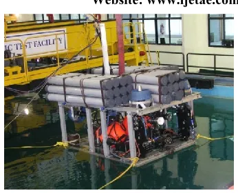
Fig.1.View of ROSUB 6000 system deployed from ship

International Journal of Emerging Technology and Advanced Engineering

383

The ROSUB system was tested up to maximum 5289m depth in Central Indian Ocean Basin. Fig.1 shows the overview of the ROSUB system.

The ROV and the TMS are docked together and launched from the mother vessel using the LARS. A 7000 m of electro-optic umbilical cable is housed in a hydraulic deck storage winch and its operation is synchronized with the LARS. The LARS handles the ROV-TMS system and transfer the load to the umbilical cable it below the splash zone. As the system reaches the desired depth, ROV is undocked out of the TMS. The ROV is propelled by thrusters and can be operated in any desired direction from the pilot command from the ship. Manipulators are used to carry out subsea intervention tasks. After the completion of the subsea task, the ROV shall be docked back to the TMS system and TMS-ROV is recovered back to the ship. The major specification of the ROV in ROSUB 6000 is given below in TABLE I.

Table I

ROSUB 6000 SPECIFICATIONS

Diving depth 6000 m

Size (Lx H x W) 2.6 x 1.9 x 2 m

Mass 3780 kg in air (-20 kg in water)

Payload Up-to 150 kg

Propulsion Seven BLDC Electrical thrusters

Power 6.6. kV, 460 Hz

Cameras Color, Monochrome and still camera

Lights LED and Halogen lights

Speed 2 knots

Navigational sensors

Inertial Navigational System aided with Doppler Velocity Log, Depth sensor and Underwater positioning system

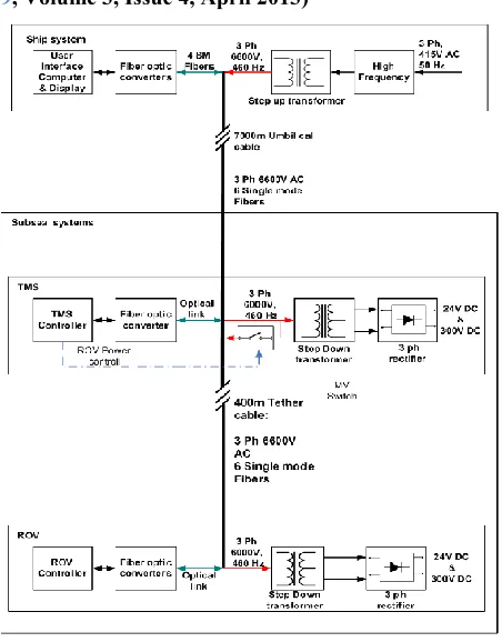
Fig.2.Electrical and control architecture of the ROSUB 6000 system

Fig.2 indicates the power and control system architecture of the ROSUB system in the TMS, ROV and the ship. Ship power at 415 V and 50 Hz is transformed into 6600 V and 460 Hz using a standard frequency converter and a step up transformer. Electro-optical connectivity between the ship and TMS is achieved by 7000 m umbilical cable. The connectivity between TMS and ROV is realized by the 400m long electro-optic tether cable. Subsea power converters are used in the TMS and the ROV, which consist of step down transformer and rectifier to convert the power into 24V and 300V DC for the subsystems. The communication between ROV and ship control systems is established using a single mode fiber optic telemetry system with wave length of 1310nm in uplink and 1550nm wave length in downlink [5].

II.ROV DYNAMICS

2.1 ROV Kinematics

International Journal of Emerging Technology and Advanced Engineering

384

2.1.1 Linear Velocity Transformation

The vehicle’s flight path relative to the earth-fixed coordinate system is given by a velocity transformation equation (1) [6]:

̇ (1)

Where J1 (η2) is a transformation matrix which is related

through the functions of the Euler angles. It is given by:

[

]

Where roll ( ), pitch ( ) and Yaw ( ).

2.1.2 Angular Velocity Transformation

The body -fixed angular velocity v2= [p q r]T and Euler rate

vector (2):

̇

Where

[

⁄ ⁄

]

Where s. = sin (.), c. = cos (.) and t. = tan (.)

2.2 ROV Kinetics

The dynamic model of the ROV is developed with the Newton–Euler formulation using laws of conservation of linear and angular momentum. The equations of motion of the vehicle are highly nonlinear and coupled due to hydrodynamic forces which act on the vehicle. The equations of motion of an underwater vehicle having six degrees of freedom with respect to a body-fixed frame of reference can be represented as mentioned in equation (3) [6]:

̇ (3)

Where

| |

MRB and CRB(v) are the rigid body mass matrix and

centripetal matrix, respectively. MA and CA(v) are the

added mass matrix and the matrix, respectively. DL and

DQ|v| are the linear and quadratic drag matrices,

respectively. g( ) is the resultant vector of gravity and buoyancy. The Coriolis and centripetal terms are negligible due to low vehicle speed of ROV maneuvering.

Thus, Major forces acting on the vehicle are due to added mass and damping forces, which are computed with respect to body frame velocity and acceleration.

2.2.1 Approaches for Underwater Vehicle Dynamics The motions of underwater vehicles exposed to ocean currents are usually modeled in six degree of freedom (DOF) by applying Newton’s second law [6].

The Linear hydrodynamic forces acting on the vehicle are given by the equations (4) – (6):

[ ̇ ̇

̇ ] (4)

[ ̇ ̇

̇ ] (5)

[ ̇ ̇

̇ ] (6)

The angular hydrodynamic moments acting on the vehicle are given by the equations (7) - (9):

̇ ( ) ̇ ̇

[ ̇ ̇ ] (7)

̇ ̇ ̇ ̇

[ ̇ ̇ ] (8)

̇ ( ) ̇ ̇

[ ̇ ̇ ] (9)

where X, Y, Z, K, M and N are the forces and moments acting on the vehicle in six degree of freedom. Even though precise instrumentation are available for measuring linear and angular changes[13] of the vehicle, the equations are very sensitive to centre of gravity (Xg, Yg, Zg), mass with added mass (m) and inertia due to mass and added mass (Ix, Iy, Iz) parameters [8]. Accurate determination of these parameters are a challenging and unsuitable for variable configuration vehicles [7, 8].

International Journal of Emerging Technology and Advanced Engineering

385

characterized by slow velocities and modest attitude changes typical of this class of work class under water vehicles [14].

III.NEED FOR DYNAMIC PLANT MODEL

The design of motion control algorithm for under water vehicles is aimed in attaining high performance in terms of precision, agility and optimization of the thruster action. Many different control methods have been proposed to handle the uncertainties accounting hydrodynamic parameters and external disturbances [10, 13, and 15]. The aim of the control strategy is to develop a nominal vehicle model and an estimate of the dynamic equation parameters required for both control and state estimation purposes [16]. Performance improvements in Guidance, Navigation and Control (GNC) in the ROSUB 6000 system is required to execute tasks such as high precision hovering in proximity of the sea bed. This requirement motivated a deeper investigation in the methodologies for hydrodynamic modeling and identification of vehicle parameters.

3.1 Estimation of Hydrodynamic Parametrs Conventional Methods

Conventional hydrodynamic derivative identification methods involves towing tanks trials of the vehicle itself in Planar Motion Mechanism (PMM) or using scaled down model of the vehicle. PMM methods [6] are costly and time consuming. Moreover, they are not suitable for variable configuration vehicles where the experiment needs to be repeated after any modification for payloads. Scaled down models test methods involve estimating the hydrodynamic coefficients of the scaled down model using free decay pendulum motion tests and the hydrodynamic parameters are identified by analyzing the time history of motion [15, 17]. By applying laws of similitude, hydrodynamic parameters of the scaled model can be scaled up to predict the corresponding values for full scale vehicle. During the tests the model has to move multiple times faster than the real vehicle [18]. This poses practical difficulties in handling the system while carrying out the pendulum decay tests. Added mass is analytically computed using strip theory [19] and are prone to inaccuracies as they involve

more engineering judgments. Silvestre et al [20] analyzed the two afore said conventional methods and they estimated an error in the estimate of some of the hydrodynamic parameters up to 50%.

3.2 Proposed Vehicle Fly-Test

Proposed practical approach consists of two steps,

a. Estimation of vehicle drag coefficients by constant speed tests for a range of velocities.

b. Estimation of moment of inertia due to added mass by subjecting the vehicle to sinusoidal motion with reasonable acceleration.

Based on the reported experimental studies of underwater vehicle dynamics and control [21, 22], ROSUB 6000 vehicle model is optimized based on the following assumptions,

 Vehicle body fixed frame is coincident with the rigid body Centre of Mass.

 Vehicle body fixed frame aligns with principal axes of inertia.

 Vehicle has top-bottom, port-starboard and fore-aft symmetries.

 Vehicle is moving with moderately slow velocities and undergoing modest attitude changes [6].

By means of the assumptions, off diagonal entries, coupling terms, tether dynamics are eliminated. The decoupled equations of motion for the ROV moving through a fluid in the body frame are written as [11, 13]. These form the basis of DTMB equations (10):

̇ | |

(10)

Where i correspond to each DOF, Ti (t) is the net control force, mi is the effective mass which includes vehicle mass

and added mass, dQ and dL terms are quadratic and linear

components of hydrodynamic drags, bi is the buoyancy.

International Journal of Emerging Technology and Advanced Engineering

386

motion where the rigid body is only moving in one direction at a time. We assume that the motion in the other five DOF is negligible [15, 19].

This paper presents the non-linear model-aided PD algorithm implemented for automatic heading control of the ROSUB 6000 vehicle. Experimental identification of a finite-dimensional dynamical plant model has been carried out. Experiments were performed to identify the de-coupled single degree of freedom plant dynamic model in the heading DOF. The identified vehicle parameters were used in PD control algorithm for achieving a high performance closed loop heading control.

IV.ROSUB 6000 ROV

The ROSUB 6000 ROV is a fully actuated vehicle equipped with seven Brushless Direct Current (BLDC) motor thrusters with the vehicle freedom in all the six degrees. Two thrusters each are used for longitudinal and lateral position control, three thrusters for vertical and two thrusters for forward and reverse functions. The thrusters with 214 kgf thrust are driven by BLDC motors and they feature light weight and high efficiency of operation.

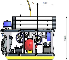
Fig. 3 ROSUB with temporary buoyancy and dimensions (side view)

The BLDC motors are operated by power electronics controller housed in pressure rated enclosure. The motor controllers are driven from a 300V DC in ROV. The thrusters are full ocean depth rated, oil filled and pressure compensated. The dimensions of the ROV with temporary buoyancy packs are shown in Fig. 3 and 4.

Fig. 4 ROSUB with temporary buoyancy and dimensions (top view)

4.1 ROV Controller

The National Instruments cFP-2220 controller is an industrial 400 MHz processor runs with VxWorks real time operating system (RTOS) for intelligent distributed applications [23]. The Controller runs with NI LabVIEW Real-Time software module for control, data logging, and signal processing. The controller is suitable for applications requiring industrial-grade reliability, stand-alone data logging, analog processes, PID control loops, actuating field devices, perform real-time analysis and simulation, log data, and communicate over serial and/or Ethernet ports. A RS-232 serial port and Ethernet ports are used to interface with external systems. The analog Input and output module NI-cFP-AIO-610 consists of four analog inputs and four analog outputs. Four analog (voltage or current) input channels has ranges up to ± 30 V or ± 20mA. Four analog voltage outputs with ±10 V range with 12-bit resolution and 1.4 kHz hardware update rate [24]. Two analog output modules are interfaced with thruster controllers to control its speed.

International Journal of Emerging Technology and Advanced Engineering

387

Table II

SENSOR USED IN ROSUB 6000 SYSTEM

Vehicle data Sensor Accuracy Update rate

Depth Para scientific 0.01% 1 Hz

XYZ velocity RDI 600kHz 0.3 % 1 Hz

Roll, Pitch

Heading PHINS 0.01deg 20 Hz

4.2 IDENTIFICATION OF VEHICLE PARAMETERS

4.2.1 Thruster Characteristics

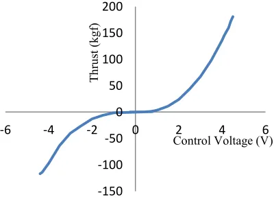
The non-linear thruster characteristics are identified by experiments at in-house test facility [25, 26]. Thruster is mounted in a suitably designed fixture with a provision to measure the thrust generated in water. Thruster control command is applied from -5V to +5VDC and the thrust produced in either direction are recorded. Fig. 5 shows the thruster characteristics are identified using 8015B thruster. The non-linear thruster behavior is recorded and a lookup table is generated and implemented in the ROV on-board real time controller. The experiments were done with the assumption that the advance velocity Va of the fluid [19]

through the thruster is negligible even though the condition departs from an unbounded open water body.

Fig. 5. Indentified performance characteristics of ROSUB thruster.

4.2.2 Test Facility and Constraints

Experiments were carried out in in-house test facility which involves a tank of dimensions 15m (L) x 9m (W) x 7m (D) and equipped with an overhead crane of 3000 kg.

The following were the constraints in carrying out the parameter identification requirements in the vehicle,

a. As the fluid is bounded, boundary induced effects such as refracted waves were observed.

b. Mass of the actual vehicle is 3700 kg. Due to handling limitations, the syntactic foam was replaced with make-shift buoyancy thus reducing the vehicle weight to 2600 kg.

c. Parameter identification could be done only for the heading DOF due to the limitation in the tank dimensions.

d. When the thruster characteristics identification is done, the operation of the thrusters sets the tank water in motion and thus resulted in advance velocity for thruster blades [19].

4.2.3 Plant Parameter Identification for Heading DOF

The moment acting in heading DOF is given the equation (11) [16]:

̇ | | (11)

Where I - Mass moment of inertia due to vehicle and added mass; v - heading velocity and T - torque.

Parameter identification involves determining the following parameters for the heading DOF.

a. Moment of inertia due to Added mass.

b. Linear component (DL) and quadratic component (DQ)

of drag force. To realize this,

1. Constant control command inputs are given to lateral thrusters of the ROV to identify hydrodynamics drag parameters.

2. Sinusoidal command is given to lateral thrusters to identify the Moment of inertia due to Added mass.

-150 -100 -50 0 50 100 150 200

-6 -4 -2 0 2 4 6

T

hru

st (

kg

f)

International Journal of Emerging Technology and Advanced Engineering

388

V.TESTING AND DETERMINATION OF PLANT PARAMETERS

5.1 Drag Parameters Identification using Constant Velocity test

The test was conducted to identifying the drag parameters of the vehicle in the heading DOF. Constant speed commands are given to the lateral thrusters of the vehicle and the steady state heading velocity responses is logged. The control signal corresponding to the required thrust is taken from the identified thruster characteristics. The torque required to move the vehicle at the specific heading velocity is the energy required to overcome the drag forces at that specific velocity. The torque recorded is the sum of linear drag DL and quadratic drag DQ forces. Fig. 6 shows

the steady state angular velocity recorded when a control command of 1.55 V is given to both the lateral thrusters. This experiment is repeated for various values of torque and the corresponding steady state heading velocities are noted in TABLE III.

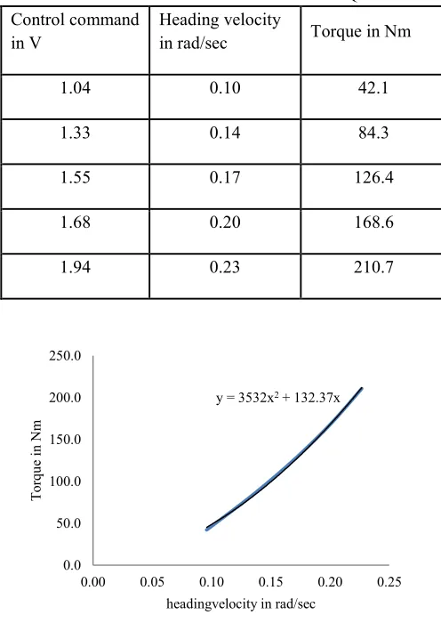
The logged data of heading velocity and torque due to the drag are plotted as shown in Fig. 7 and curve fitting is carried out. The curve generated value for DL and DQ are

used in the control algorithm for heading DOF.

Fig. 6 Velocity profile recorded when 1.55V control command is applied to lateral thrusters.

Table III

HEADING ANGULAR VELOCITIES VS TORQUE Control command

in V

Heading velocity

in rad/sec Torque in Nm

1.04 0.10 42.1

1.33 0.14 84.3

1.55 0.17 126.4

1.68 0.20 168.6

1.94 0.23 210.7

Fig. 7 Heading velocity versus torque in heading DOF

5.2 Determination of Added Mass Parameters

Due to the handling limitations, syntactic foam of ROV is replaced with temporary buoyancy packs. Required buoyancy correction was carried out before conducting the test. ROV vehicle mass was measured using a load cell with 0.02% accuracy. The mass of ROV is found to be 2604 kg. Fig. 8 shows the ROV with temporary buoyancy is showed.

0.00 0.04 0.08 0.12 0.16 0.20

1200 1250 1300 1350

H

ead

ing

v

el

o

ci

ty

(

rad

/s)

Time in seconds

y = 3532x2 _{+ 132.37x}

0.0 50.0 100.0 150.0 200.0 250.0

0.00 0.05 0.10 0.15 0.20 0.25

T

orq

ue

in

Nm

International Journal of Emerging Technology and Advanced Engineering

389

Fig. 8 ROV is being launched in tank with temporary buoyancy

The test was conducted to identify the added mass of the vehicle in the heading degree of freedom. The added mass/moment of inertia of underwater vehicles operating below the water surface is independent of wave excitation amplitude and frequencies [6, 19]. A sinusoidal control command (with peak torque corresponding to specific steady state heading velocity) is given to the lateral thrusters of ROV and the heading velocity of the vehicle is recorded. Fig.9 shows a sinusoidal control command with 1/40 Hz frequency given to the lateral thrusters with the amplitude of given command signal corresponding to +1.55V to -2.2 V in the forward and reverse directions respectively.

Fig.9. Sinusoidal control command applied to lateral thrusters

This corresponds to 102.9 Nm torque required to attain a steady state heading velocity of 0.17 rad/s. But the measured peak sinusoidal angular velocity is 0.12 rad/s. (shown in fig10). The measured heading velocity is less than the velocity recorded during the steady state velocity test. This indicates that the vehicle requires more torque to

overcome the Inertia due to mass and added mass of vehicle.

Fig.10. Heading velocity recorded when 1/40 sine signal command (1.55V) is given to lateral thrusters

To achieve the commanded velocity profile, a thrust component equal to mass moment of inertia (I) multiplied by angular acceleration (α) is to be added to the sinusoidal velocity (thrust) command. Torque difference between the thrust required for steady state velocity and sinusoidal velocity for obtaining the specific heading velocity is due to moment of inertia. The amplitude control command is increased until the peak heading velocity reaches to the same velocity when steady state test was carried out. Fig. 11 shows that, a sinusoidal control command with 1/40 Hz frequency is given to the lateral thrusters with the amplitude of given signal corresponds to +2.00V to -2.51V in the forward and reverse directions and corresponding to 126.42 Nm torque.

Fig.11. Sinusoidal control command applied to lateral thrusters

-2.50 -1.50 -0.50 0.50 1.50

1944 1994 2044

Co

ntro

l v

olt

ag

e

in

V

Time in Seconds

-0.15 -0.10 -0.05 0.00 0.05 0.10 0.15

1944 1994 2044

Hea

din

g

velo

city

in

r

ad

/s

Time in Seconds

-2.50 -1.50 -0.50 0.50 1.50 2.50

2300 2320 2340 2360 2380 2400

C

on

tr

ol

v

ol

ta

ge

in

V

International Journal of Emerging Technology and Advanced Engineering

390

Peak heading velocity of 0.17rad/s is obtained when a torque of 227.56Nm is applied and the same can be seen from fig.12.

Fig.12. Heading velocity recorded when 1/40sine signal command (2.00V) is given to lateral thrusters

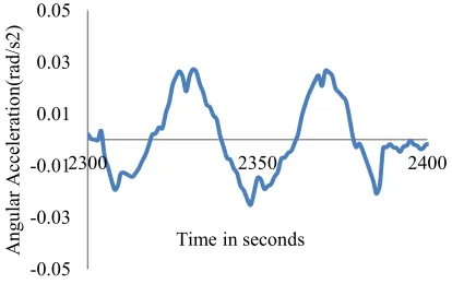
The measured peak sinusoidal angular velocity is 0.17rad/s. The torque difference is 101.36 Nm from steady state velocity test and Sinusoidal test for attained velocity of 0.17 rad/s. The torque is product of the moment of inertia (due to vehicle mass and added inertia) and angular acceleration. Peak heading acceleration is recorded (0.02 rad/s2_{) during this test as shown in Fig. 13. The mass}

moment of inertia due to added mass is found to be 2708.1 kg m2_.

Fig.13. Angular acceleration logged when 1/40Hz sine signal applied with 2.00V amplitude.

The following TABLE IV shows that the experimental results of the Plant parameters computed from the steady state velocity test and transient velocity test.

Table IV ROV PLANT PARAMETERS

Drag parameters _{Mass moment of inertia (kg} m2₎

DQ DL

3532 132 5057

VI.DESIGNANDIMPLEMENTATIONOFHEADING CONTROL

Generally, PD and PID controls are used in ROV control [11]. An ROV is a hydro dynamically damped system and stability is required for smooth maneuvering in low speeds and hence PD controller is chosen. Identified vehicle parameters are used in the above equation and closed loop control is implemented for the heading DOF. PHINS does not generally provide angular rates but provides earth reference velocity and Euler angles. From the available data, body frame angular velocity is computed using angular transformation [6] for heading control.

6.1 Heading Control Loop Implementation with Vehicle-Model and PD Control

ROV closed loop control equation for heading is given by the equation (12):

̇ | |

̇ (12)

Where, v is the heading velocity (rad/sec) with respect to body frame. The equations involve proportional and derivative components in addition to the model driven moments. The heading control loop algorithm is implemented using LabVIEW as shown in fig.14. The control algorithm is based on PD control supplemented by vehicle dynamic model. The output of the vehicle dynamic model is the sum of the drag force based on the vehicle body frame velocity and the added mass. The output of the proportional control is based on the difference in offset between the set and the actual vehicle heading.

-0.20 -0.15 -0.10 -0.05 0.00 0.05 0.10 0.15 0.20

2300 2350 2400

He

ad

in

g

V

elo

cit

y

(ra

d/s)

Time in seconds

-0.05 -0.03 -0.01 0.01 0.03 0.05

2300 2350 2400

A

ng

ular A

cc

elera

ti

on

(ra

d/s2

)

International Journal of Emerging Technology and Advanced Engineering

391

The output of the derivative control is based on the change in the vehicle velocity.

PD Controller

+

-+

Inertial Navigation

System Input command

ROV

Thrust allocation

Control output

Velocity transformation Surge, Sway & Heave

Roll, Pitch & Heading

ROV Dynamics

+

Fig.14. ROV heading control algorithm

6.2 PD Control Tuning and Testing

The damping ratio for a closed loop system is shown in the equation (13) [11]:

_√ (13)

Where, m is the mass of the vehicle, kp is the proportional

constant, kd is the derivative constant and ς is the damping

ratio of closed loop system. The Kp and Kd are tuned based on the trial error methods [27] so as to obtain the optimal system response. The values of Kp and Kd are driven based on the classical rule for linear closed loop systems.The value of damping ratio is chosen to 0.7 which corresponds to an under-damped system [6, 19]. With the vehicle-model algorithm in the operation, the algorithm is tuned for a range of proportional and derivative constants. The proportional and the derivative constants are thus found to be as follows, Kp = 100; Kd = 710.

6.3 Control Algorithm Performance Results

The ROV was at a heading 90 deg and the heading set point is given as 200 deg. The response of the algorithm for attaining the set value is recorded and shown in fig. 15.

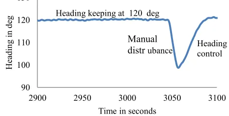
The ROV heading algorithm is tested for its performance at different set points. Fig. 16 shows the heading loop response when predetermined heading command was given. The vehicle is kept at a constant heading of 120 deg and displaced to 100 deg. manually. The system response is shown in Fig.17.

Fig. 15 Heading tracking with given set command

Fig. 16 Heading loop response when it reaches 120 deg from 20 deg

Fig. 17 Heading keeping when external disturbance occur

1.00 1.50 2.00 2.50 3.00 3.50 4.00

1170 1220 1270

He

ad

in

g

in

ra

d

Time in Seconds

heading in rad

heading set in rad

15 35 55 75 95 115 135

2700 2750 2800

He

ad

in

g

in

d

eg

time in seconds

90 100 110 120 130

2900 2950 3000 3050 3100

He

ad

in

g

in

d

eg

Time in seconds Heading keeping at 120 deg

Manual

International Journal of Emerging Technology and Advanced Engineering

392

It can be seen that for tests that the system had a response time of 25 and 26 seconds for a disturbance in angles of 100 and 80 deg respectively. The corresponding time constant is calculated [19] to be 20 and 22 seconds. The results are found to comply with Nomoto model tests [19] where in the time constant of 25 seconds was observed for under water vehicles [16].

VII. CONCLUSION

ROV vehicle parameters are identified for heading degree of freedom using steady state velocity and transient state velocity test. Non-linear model based PD approach algorithm was implemented with identified vehicle parameters and the heading control functionality was tested. Heading keeping is tested when external disturbance introduced in the vehicle. Response of the heading control is satisfactory maintaining heading with in ± 0.6 degree. Heading control of ROV will be further tested and optimized with the actual syntactic foam buoyancy in the unbounded medium. Parameter identification of surge, sway, heave, roll and pitch will be identified similarly.

ACKNOWLEDGEMENTS

The authors gratefully acknowledge the support extended by the Ministry of Earth Science, Government of India, in funding this research. The authors also wish to thank the members of Submersibles & Gas Hydrates group for their contribution and support. Authors wish to thank Prof. N Kumaravel, Head of ECE dept and Dr. P Sakthivel, associate professor for their encouragement and support.

REFERENCES

[1] Bruno Sicilian, Oussama Khatib, Underwater Robotics, Springer Handbook of Robotics, (New York: Springer, 2008) 987-1007. [2] Manecius Selvakumar J, Ramesh R, Subramanian AN,

Sathianarayanan D, Harikrishnan G, Jayakumar VK, Muthukumaran D, Murugesan M, Chandresekaran E, Elangovan S, Doss Prakash V, Vadivelan A, Radhakrishnan M, Ramesh S, Ramadass GA, Atmanand MA, Technology tool for deep ocean exploration – Remotely Operated Vehicle, Twentieth International Offshore (Ocean) and Polar Engineering Conference., 2010.

[3] N Vedachalam, R Ramesh, S Ramesh, D Sathianarayanan, A N Subramaniam, G Harikrishnan, SB Pranesh, VBN Jyothi, Tamshuk Chowdhury, G A Ramadass, M A Atmanand, ―Challenges in realizing robust systems for deep water submersible ROSUB6000‖, International symposium on Underwater Technology, 2013.

[4] D Sathianarayanan, R Ramesh, AN Subramaniam, G Harikrishnan, D Muthukumaran, M Murugesan, E Chandrasekaran S Elangovan, V Dossprakash, A Vadivelan, M Radhakrishnan, S Ramesh, G A Ramadass, M A Atmanand, ―Deep sea qualification of Remotely Operable Vehicle (ROSUB 6000)‖, International symposium on Underwater Technology, 2013.

[5] Ramesh R, Jayakumar VK, Manecius Selvakumar J, Doss Prakash V, Ramadass GA, Atmanand MA, Distributed Real Time control systems for deep water ROV (ROSUB 6000), Proc. International Conference on Computational Intelligence, Robotics and Autonomous Systems (CIRAS), Bangalore, 2010, 33- 40.

[6] Thor I Fossen, Guidance and Control of Ocean Vehicles, (Norway : John Wiley Publication, 1994), Pages: 50-51.

[7] Conte S.M. Zanoli, D. Scaradozzi, and A. Conti, Evaluation of hydrodynamics parameters of a UUV. A preliminary study, International Symposium on Control, Communications and Signal Processing, ISCCSP, 2004.

[8] M. Caccia, G. Indiveri, and G. Veruggio, Modeling and identification of open frame variable configuration unmanned underwater vehicles, IEEE Journal of Oceanic Engineering, 25(1), 2000, 2240-2242. [9] C. Silvestre, A. Aguiar, P. Oliveira, A. Pascoal, Control of SIRENE

underwater shuttle system design and tests at sea, Proc. 17 th International Conference of Offshore and Artic, Lisbon, Portugal, 1998.

[10] D.A. Smallwood and LL Whitcomb, Preliminary experiments in the adaptive identification of dynamically positioned underwater robotic vehicles, Proc. IEEE/RSJ Int. Conf. Intelligent Robots and Systems, Maui, 2001, 1803-1810.

[11] DA Smallwood, Advances in Dynamic modeling and control of underwater robotic vehicles, Ph.D dissertation, The Johns Hopkins University, Baltimore, MD, 2003.

[12] M Gertler and Grant R Hagen, Standard equations of motions for submarine simulations, Technical report, David Taylor Naval Ship Research and Development Center, 1967.

[13] D.A.Smallwood and L.L.Whitecomb, Adaptive identification of dynamically positioned underwater robotic vehicles, IEEE Transactions on Control System Technology, Vol 11, 2003, 505-515. [14] J. N. Newman, Marine Hydrodynamics, (London : MIT, 1989). [15] M.S. Triantafyllou and F.S. Hover, Maneuvering and Control of

Marine Vessels, Department of Ocean Engineering, (USA: MIT, 2003) [16] Juan Pablo Julca Avila, Newton Maruyama, Julio Cezar Adamowski, Hydrodynamic parameter estimation of an open frame unmanned underwater vehicle, Proc. 17th IFAC World Congress (IFAC'08) Seoul, Korea, 2008.

[17] Ross and Johansen, Identification of underwater vehicle hydrodynamic coefficients using free decay tests, IFAC Conference on Control applications in Marine Systems, 2004.

[18] Eng YH, Lau WS, Seet GGL and CS Chin, Estimation of hydro dynamic coefficients of an ROV using free decay pendulum motion, Engineering Letters, 16:3, 2008.

[19] Thor I Fossen, Handbook of Marine Craft Hydrodynamics and Motion Control, (Norway: John Wiley Publication, 2011).

[20] M. Nomoto, Hattori M, A deep water ROV Dolphin 3 K, Design and performance analysis, IEEE Journal of Ocean Engineering, 11(3), 1986, 373-391.

[21] A.J. Healey, Model based maneuvering controls for autonomous underwater vehicles, ASMEJ Dynamic Systems Measurement and Control, 114(4), 1992, 614-662, 1992.

[22] T I Fossen and S I Sangatun, Adaptive control of non-linear underwater robotic systems, Proc. IEEE International Conference of Robotic Automation, Sacramento, CA, 1991.

International Journal of Emerging Technology and Advanced Engineering

393

for compact field point, Ref: 374708C-01, Feb 2009

[24] National Instruments Field point operating Instructions, cFP-AIO- 610 analog input and output module, ref: 373174C- 01, Jul 2006. [25] R. Bachmayer, L L. Whitecomb, An accurate four quadrant non-linear

dynamic model for marine thrusters: Theory, IEEE Journal of Oceanic Engineering , 25(1), 2000, 149-159.

[26] Dana R Yoeger, Cooke, J.G., Slotine, The influence of thruster dynamics on underwater vehicle behavior and their incorporation into control system design, IEEE journal of oceanic engineering, 15(3), 1990, 167-178.