Model building with multiply imputed data

29

Chapter 4

Model-Building with Multiply Imputed Data

Khuneswari Gopal Pillay1, John H. McColl2

1 _{Department of Mathematics and Statistics, Faculty of Science, Technology and}

Human Development, Universiti Tun Hussein Onn Malaysia, 86400 Batu Pahat, Johor, Malaysia, [email protected]

2 _{Department of Statistics, School of Mathematics and Statistics, University of}

Glasgow, G12 8SQ Glasgow, Scotland, United Kingdom.

Abstract. Model selection is well-known for introducing additional uncertainty which can be more severe in the presence of missing data. Model averaging is an alternative to model selection which is intended to overcome the under-estimation of standard errors that is a consequence of model selection. Model selection and model averaging were explored on multiply-imputed data sets in terms of model selection and prediction. Three different model selection approaches (RR, STACK and M-STACK) and model averaging using three model-building strategies (non-overlapping variable sets, inclusive and restrictive strategies) to combine results from multiply-imputed data sets were explored using a basic Monte Carlo simulation study on linear and generalized linear models. The results showed that the STACK method performs better than RR and M-STACK in terms of model selection and prediction, whereas model averaging performs slightly better than STACK in terms of prediction. The inclusive and restrictive strategies perform better in terms of prediction but non-overlapping variable sets performs better for model selection. In conclusion, researchers should use STACK (with non-overlapping variable sets) for analysing data with missing values to determine which variables to include when making predictions but use model averaging (with a restrictive strategy) for prediction.

30

1

Introduction

Model selection is an important part of the model-building process and cannot be separated from the rest of the analysis in choosing the best model. However, model selection is well-known for introducing additional uncertainty into the model-building process. The properties of standard parameter estimates obtained from the selected model do not reflect the stochastic nature of the model selection process [2]. This effect can be more severe in the presence of missing data. In the literature, model averaging has been proposed as an alternative to model selection which is intended to overcome the under-estimation of standard errors that is a consequence of model selection [1].

Various strategies have been proposed for building model for the imputation of missing values and then prediction of a response, depending on how auxiliary variables are treated. Auxiliary variables are variables within the original data that would not usually be included in the main analysis, but are correlated to the covariates of interest and may be used in the imputation model [4]. A restrictive strategy is including few or no auxiliary variables in both imputation and prediction models [3]. An inclusive strategy involves including numerous auxiliary variables and overlapping variable sets in both the imputation and prediction models. A strategy of using non-overlapping variable sets (an extremely restrictive strategy) is defined as not including auxiliary variables in the prediction model, but only in the imputation model, so that distinct variable sets are considered for the imputation and prediction models.

The main objective of this research is to compare various variable selection approaches for the prediction model and model averaging in terms of model selection and prediction. Three different model selection approaches will be explored in order to identify the best method of model selection with multiply-imputed data sets. The three approaches are backward stepwise regression using Rubin's rules (RR), the stacked imputation method (STACK) [7] and a modified stacked imputation method (M-STACK). Model averaging will also be explored and compared with the model selection methods in terms of prediction, as indicated by mean squared error of prediction (MSE (P)). A basic Monte Carlo simulation design will be used to explore these approaches with a fixed lattice of test values in the covariate space being used to evaluate MSE (P).

2

Model Selection and Model Averaging Methods

2.1 Design of Simulation

The general multiple linear regression model considered (true model) was

0 1 1 2 2

i i i i

31 whereY is the response variable, X's are explanatory variables, 's arecoefficients/ parameters of the model, is an error term and n is the number of observations. The logistic regression model considered (true model) was:







00 1111 2222



exp

( 1)

1 exp

i i i

i i

i i i

X X

P P Y

X X

   

   

  

  

    , i1, 2,...,n (2)

Equation (2) can be re-written as:

0 1 1 2 2

i i i i

logit P  X  X  (3)

whereY is a binary response variable, which can only take the value 1 or 0,

ln 1 i i i P logit P P     _ 

 and Pi is the probability of success (in the range 0 to 1). X(X X X₁, ₂, ₃)values were simulated from a multivariate normal distribution with fixed zero means and a specified covariance matrix. Y values were created based on Equation (1), the simulated X₁ and X₂ values and, for linear models, the error terms simulated from 2

(0, ) N _

where 2 1 ,1,16 16 

  . In all simulations, ₀ ₁₂1. X₁andX₂ represent covariates in a prediction model for the response Y, with some values of X₂ (but not X₁) missing. X₃is an auxiliary variable, primarily intended to use in the imputation model for X₂. The covariance matrix for

X(X X X₁, ₂, ₃) is therefore

23

23

1 0 0

0 1 0 1               (4)

where₂₃₃₂ denotes the correlation between X₂ and X₃,

12 13 0

   and₂₃ 0.75, 0.5, 0.25, 0, 0.25, 0.5, 0.75 . The

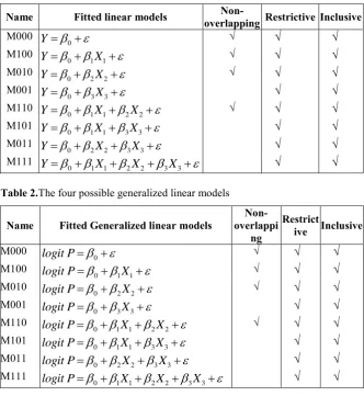
32 There were four possible models for linear and generalized linear models as listed in Table 1 and Table 2.

Table 1.The four possible linear models

Name Fitted linear models _overlapping Non- Restrictive Inclusive M000

0

Y  √ √ √

M100

0 1 1

Y  X  √ √ √

M010

0 2 2

Y  X  √ √ √

M001

0 3 3

Y  X  √ √

M110

0 1 1 2 2

Y X  X  √ √ √

M101

0 1 1 3 3

Y X  X  √ √

M011

0 2 2 3 3

Y  X  X  √ √

M111

0 1 1 2 2 3 3

[image:4.595.130.463.199.561.2]

Y X  X  X  √ √

Table 2.The four possible generalized linear models

Name Fitted Generalized linear models overlappi Non-ng

Restrict

ive Inclusive M000

0

logit P  √ √ √

M100

0 1 1

logit P X  √ √ √

M010

0 2 2

logit P  X  √ √ √

M001

0 3 3

logit P  X  √ √

M110

0 1 1 2 2

logit P X  X  √ √ √

M101

0 1 1 3 3

logit P X  X  √ √

M011

0 2 2 3 3

logit P  X  X  √ √

M111

0 1 1 2 2 3 3

logit P X  X  X  √ √

The "norm.nob" imputation method in MICE package [6] was used to impute any missing observations of X₂using the auxiliary variableX₃. The imputation model used in both restrictive strategy and non-overlapping variable sets was

2i ˆ0 ˆ3 3i ˆ4 i

X   X Yh (5)

33 2i ˆ0 ˆ1 1i ˆ3 3i ˆ4 i

X   X  X Yh (6)

0 ˆ

 ,ˆ₁,ˆ₃andˆ₄were estimated from the complete cases using least

squares, and h_iwas a random error from _ˆ2

(0, h)

N  .

2.2 Model Selection Approaches

There are three model selection approaches to combining results from multiply-imputed data sets. The three approaches are backward stepwise regression using Rubin's rules (RR), the stacked imputed data set method (STACK) and a modified stacked imputed data set method (M-STACK). The RR method is considered as gold standard approach but it is more computationally demanding when repeated analyses are required. Therefore, the STACK method was proposed as a sensible alternative to RR method for repeated analyses [7]. The STACK method use backward stepwise selection approach for variable selection. The backward stepwise selection approach is often criticised. A modified version modified version of the stacked imputed data sets method (M-STACK) is proposed as an alternative to STACK and RR.

2.2.1 Backward stepwise regression using Rubin’s Rules (RR)

The first method is backward stepwise regression using repeated use of Rubin's rules (RR). The simple backward stepwise regression using Rubin's rule for four models (M000, M100, M010, M110) are as following [5]:

Step 1:Run model M110 for each imputation, store



ˆ andcov( )ˆ ˆ .

Step 2:Check 1 1 ˆ

1.96

. . ( )

e s e



  and

2

2 ˆ

1.96

. . ( )

e s e



  .

Step 3:If both parameters are significant, record count of 1 for fitting model M110 and calculate MSE(P) using  .

Step 4:If ₂is not significant, run model M100 for each imputation. Store ˆ



andcov( )ˆ ˆ .

Step 5:Check 1 1 ˆ

1.96

. . ( )

e s e



34 Step 6: If ₁is not significant, run model M010 for each imputation. Store

ˆ



andcov( )ˆ ˆ .

Step 7: Check 2 2 ˆ

1.96

. . ( )

e s e



  . If 2is significant, record count of 1 for fitting model M010 and calculate MSE(P) using .

Step 8: If ₂is not significant, run model M000 for each imputation. Store ˆ



andcov( )ˆ ˆ . Record count of 1 for fitting model M000 and calculate MSE(P) using .

2.2.2 STACK

The second method uses the stacked imputed data sets with weighted regression (STACK) [7]. In this method, D imputed data sets will be stacked for the nindividuals which yields one large dataset of lengthD_n. A fixed weight will be applied to all individuals to correct the standard errors. Although [7] proposed three possible weights, but they claimed

3

W was the best. Therefore, weight W3will be used in this research. The considered weight

W

3

is

(1 _i)

i f w D   (7)

where f_iis the fraction of missing data for variableX_iand it is calculated as

i i

number of missing data for variaable X f

n

 (8)

The largest f_iwill be used across all the variables in the context of more variables with missing data in a model. Weighted regression analysis will be carried out using stacked imputed data.

The essential assumption of the STACK method is that fraction of missing data equals fraction of missing information. This assumption yields the weight W3 in MCAR mechanism. It was pointed out that the

3

35 prediction model are uncorrelated in the setting of non-overlapping variable sets.

In this research, the model selection is carried out on stacked data using model selection criteria (AICc and BIC) rather than the backward stepwise selection approach. Although the original version of STACK method proposed by [7] is using backward stepwise selection approach for variable selection, this research is interested in using model selection criteria for model selection. All possible models are fitted to the single stacked dataset and a best model is selected using model selection criteria. Then, the selected best model will be fitted for each imputed dataset separately and the parameter estimates will be combined using RR. The number of times each possible model is selected via each selection criterion was calculated. The MSE(P) was calculated for the combined parameter estimates using RR.

2.2.3 Modified STACK (M-STACK)

The third method is a modified version of the stacked imputed data sets method with weighted regression (M-STACK). All possible models are fitted to the single stacked dataset and a best model is selected using model selection criteria (same as STACK). In this method, however, the final estimates of the parameters are taken to be the ones given by the analysis on the stacked dataset; this avoids the final, potentially computationally-expensive, step of STACK that involves refitting the models in each imputed dataset. This approach is justified by Appendix A of [7], where it is shown that this estimator has reasonable large-sample properties. The MSE(P) was calculated using the final estimates of the parameters of the stacked dataset.

2.3 Model Averaging

36 1 exp 2 exp 2 M I w I              



M M M M (9)

whereI_M is model selection criterion for model M as in Equation (1) and

1 1 M w  



M M

. The estimate of a parameter _pis

( , ) 1

ˆ M ˆ

p w p

 







M M

M

(10)

where



ˆ_{( ,pM)}is the estimate of _punder model M for M=1,2,...,M. In this research, the modified weights will be used based on model selection criterion AICc[1,2]. A modification was carried out for calculating the weights in order to avoid numerical error. The weights w_M were calculated as 1 exp 2 exp 2 M I w I                



l l M M M M (11) where 1 1 M M  



l lM M

with l_M is log-likelihood function of model

M

for

=1,2,...,M

37

3 Results

A basic Monte Carlo simulation study was conducted based on the simulation design discussed earlier, for both linear and generalized linear models. The analysis was carried out for every combination of 2

, , n m_ and covariance matrix. The performance of three model selection methods and model averaging were compared using mean square error of prediction.

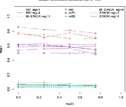
3.1 Linear Models using Non-overlapping Variable Sets

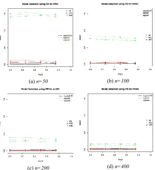
For the RR approach, the chances of choosing model M110 increases as sample size and ₂₃increases whereas the chances of choosing model M110 decreases as _and missing percentages increase. Fig. 1(a), Fig. 1(b), Fig. 1(c) and Fig. 1(d) show the MSE(P) for best model selected using RR approach for each ₂₃, _, missing percentages and sample

38

(a) n=50 (b) n=100

(c) n=200 (d) n=400

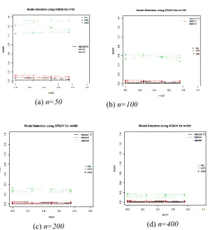
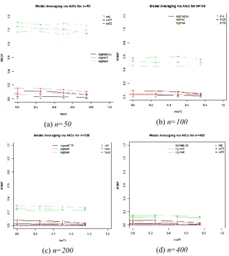
[image:10.595.135.454.149.499.2]

39 (a) n=50 _{(b) n=100}

(c) n=200 (d) n=400

Fig. 2.MSE(P) for best model selected via AICc using STACK for each₂₃,_, missing percentages and sample sizes.

As missing percentages, sample size and ₂₃increase, the chances of choosing the true model M110 using method STACK increases. Imputation improves the choice of true model M110 as sample size and

23

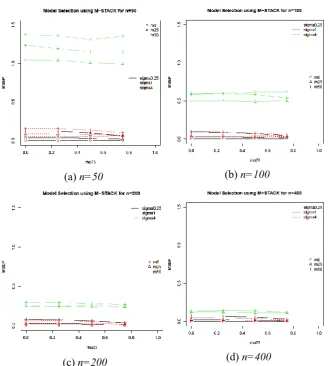
[image:11.595.144.452.142.472.2]

40

(a) n=50 (b) n=100

(c) n=200 (d) n=400

Fig. 3.MSE(P) for best model selected via AICc using M-STACK for each₂₃,_ , missing percentages and sample sizes.

[image:12.595.130.459.147.514.2]

M-41 STACK decreases as sample size increases. The effects of error variance reduce as sample size increases.

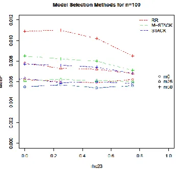
Fig. 4 shows comparison between all three model selection methods (RR, STACK and M-STACK) for each₂₃,_, missing percentages and n=100.It shows that high correlation between variable X₂and X₃ improves predictions. For larger error variance, MSE(P) for best model selected using STACK and M-STACK are lower than RR approach. Whereas the MSE(P) for best model selected using RR approach and STACK are lower than M-STACK for_ 1. The results showed that STACK performs better than RR approach and M-STACK method for all values of error variance, _and sample size in general. Therefore, STACK can be chosen as best model selection method.

Fig. 4. Comparison between model selection methods for each₂₃,_, missing percentages and sample sizes.

[image:13.595.186.396.339.518.2]

42

(a) n=50 (b) n=100

(c) n=200 (d) n=400

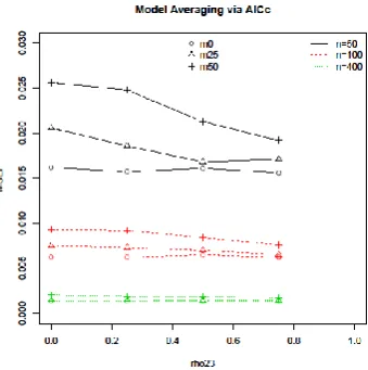
Fig. 5.MSE(P) for model averaging via AICc for each₂₃,_, missing percentages and sample sizes.

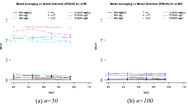
[image:14.595.131.460.149.517.2]

43

[image:15.595.132.462.151.333.2]

(a) n=50 (b) n=100

Fig. 6. Comparison between model averaging and model selection (STACK) via AICc for each₂₃,_, missing percentages and sample sizes (n=50 and n=400).

3.2 Generalized Linear Models using Non-overlapping Variable Sets

For RR approach, the chances of choosing true model M110 decreases as missing percentages increases whereas it increases as sample size increases. After imputation, the chances of choosing true model M110 increases as₂₃increases. Fig. 7(a) shows the MSE(P) for best model selected using RR for each₂₃missing percentages and sample sizes. As sample size and ₂₃increases, the MSE(P) for best model selected using RR approach decreases. The effects of missing percentages on MSE(P) for best model selected using RR approach reduces as sample size increases.

44

(a) RR (b) STACK

Fig. 7.MSE(P) for best model selected using RR and STACK.

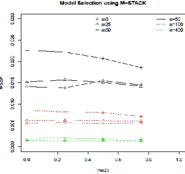
Fig. 8.MSE(P) for best model selected using M- STACK.

For M-STACK method, the chances of choosing true model M110 decreases as missing percentages increases whereas the chances of choosing true model M110 increases as sample size and ₂₃increases. Fig. 8 shows the MSE(P) for best model selected using M-STACK for each

23

[image:16.595.134.459.155.332.2] [image:16.595.200.382.372.542.2]

45 The effects of missing percentages on MSE(P) for best model selected using M-STACK reduces as sample size increases.

[image:17.595.206.379.369.534.2]

Fig. 9 shows comparison between all three model selection methods (RR, STACK and using M-STACK) via AICc for each 23, missing percentages and n=100. It shows that the MSE(P) for best model selected using using STACK is lower than RR approach and M-STACK for all ₂₃, missing percentages and sample size. For model averaging, the MSE(P) decreases as sample size and ₂₃increases. As missing percentages increases, the MSE(P) values increases. With m=0, there is no clearer difference as ₂₃increases. With missing percentages m=25 and m=50, the MSE(P) decreases as ₂₃increases. There are some difference on MSE(P) values as ₂₃, n and missing percentages increases. High correlation between variable X₂and X₃produce lower MSE(P) values in all three model selection methods.

Fig. 9.Comparison between all three model selection methods.

46 Fig. 10.MSE(P) for model averaging via AICc for each₂₃, missing percentages and sample sizes.

[image:18.595.207.377.154.325.2]

(a) n=50 (b) n=400

Fig. 11. Comparison between model averaging and model selection (STACK) for each₂₃, missing percentages and sample sizes (n=50 and n=400).

[image:18.595.133.461.382.563.2]

47 Fig.11 (b) shows comparison between model averaging and model selection (STACK) via AICcfor each 23, missing percentages and n=400. The MSE(P) for model selection using STACK is lower than model averaging. It shows that model selection using STACK performs better than model averaging in terms of prediction for large sample sizes in logistic regression.

3.3 Comparison between Model-Building Strategies

All three model-building strategies (non-overlapping variable set, restrictive and inclusive strategies) were compared for model selection (STACK) and model averaging for linear regression and logistic regression in terms of predictions. Fig. 12 shows the comparison between all three model-building strategies for model averaging and model selection (STACK) via AICc for multiply imputed data sets for each 23,, missing percentages and sample sizes, n=50 and n=400.

For _ 1and all sample sizes, there is no difference between the model-building strategies for both model selection (STACK) and model averaging. Whereas for _ 4and large sample size, there is no difference between the MSE(P) for model averaging and model selection (STACK) using all three model-building strategies. There is no effects of the negative and positive correlations of same magnitude for model averaging and model selection (STACK) with all three model-building strategies.

48 (a) Model Averagingn=50 (b) Model Selection (STACK) n=50

(c) Model Averagingn=400 (d) Model Selection (STACK) n=400

Fig. 12. Comparison between all three model-building strategies for model averaging and model selection (STACK) for multiply imputed data sets on linear regression.

[image:20.595.131.464.146.529.2]

49 variable set for all sample sizes. There are no differences between the MSE(P) values for model averaging and model selection (STACK) using all three model-building strategies for negative and positive correlations of same magnitude. The MSE(P) values of model selection (STACK) using non-overlapping variable set is lower than the MSE(P) values of model selection (STACK) using restrictive and inclusive strategies for small sample size. However, there are no differences between the MSE(P) values for model selection (STACK) using all three model-building strategies for large sample size.

(a) Model Averaging (b) Model Selection (M-STACK) Fig. 13. Comparison between all three model-building strategies for model averaging and model selection (STACK) for multiply imputed data sets on logistic regression.

4

Discussion and Conclusions

The performance and effectiveness of three methods for model selection in linear and generalized linear models were observed and compared. The effects of simulation parameters (sample size (n), missing percentages (m), the correlation between X₂and X₃(₂₃) and error variance ( 2



 ) on model selection were observed. In linear models, _has a significant effect on model selection and prediction.

[image:21.595.133.462.281.461.2]

50 model M110 more often. There is no difference between STACK and M-STACK methods in terms of selecting the true model M110 more often. Since STACK and M-STACK methods perform better than RR approach, stacked imputed data with weighted linear regression is better than RR approach applied to linear regression. The performance of the three methods can be arrange in the order STACK>M-STACK>RR for linear models. Model averaging using multiple imputation for imputing missing data performs better than STACK method for larger error variance and small sample size in terms of prediction. There is no difference between model averaging and STACK method for smaller error variance and large sample size in terms of prediction.

In the generalized linear model, STACK and M-STACK methods perform better than RR in terms of selecting true model M110 more frequently and also in terms of prediction. This shows that weighted logistic regression is better for model selection and prediction. The performance of the three methods can be arranged in the order STACK>M-STACK>RR in terms of model selection and prediction for logistic regression. Model averaging performs better than STACK method for small sample size in terms of prediction. Whereas, model selection using STACK performs better than model averaging for large sample size in terms of prediction.

MSE(P) was lowest when inclusive and restrictive strategies were used with model averaging using single and multiple imputation. MSE(P) was lowest when inclusive and restrictive strategies were used with model averaging and model selection (STACK) for both linear and generalized linear models. Negative and positive correlations of the same magnitude have the same effect on prediction for model averaging and model selection (STACK) using all three model-building strategies. There is not much difference between the restrictive and inclusive strategies in terms of prediction for model averaging and model selection. It is advisable to use the inclusive strategy to make predictions.

51 models, and also use highly correlated auxiliary variables (when available) in imputation models.

References

1. Buckland, S. T., Burham, K. P., and Augustin, N. H. (1997). Model selection: An integral part of inference. Biometrics, 53(2): 603-618.

2. Burham, K. P. and Anderson, D. R. (2002). Model Selection and Multimodel Inference: A practical Information-Theoretic Approach. Springer-verlag New York Inc., New York.

3. Collins, L. M., Schafer, J. L., and Kam, C. M. (2001). A comparison of inclusive and restrictive strategies in modern missing data procedures. Psychological Methods 6(4): 330-351.

4. Hardt, J., Herke, M., and Leonhart, R. (2012). Auxiliary variables in multiple imputation in regression with missing x: A warning against including too many in small sample research. BMC Medical Research Methodology 12: 184.

5. Little, R. J. A. and Rubin, D. B. (2002). Statistical analysis with missing data. John Wiley and Sons, Inc., New Jersey, second edition.

6. van Buuren, S. and Groothuis-Oudshoorn, K. (2011). Mice: Multivariate imputation by chained equations in r. Journal of Statistical Software 45(3): 1-31.