Efficient solution for nonlinear dynamic estimation problem with model reality differences

Efficient solution for nonlinear dynamic

estimation problem with model-reality

differences

Sie Long Kek1, Kim Gaik Tay2 and Kuan Chin Chua3

1 _{Department of Mathematics and Statistics, Universiti Tun Hussein Onn Malaysia,} 86400 Parit Raja, MALAYSIA

[email protected]

2 _{Department of Communication Engineering, Universiti Tun Hussein Onn Malaysia} 86400 Parit Raja, MALAYSIA

3 _{Department of Mathematical and Actuarial Sciences, Universiti Tunku Abdul Rahman} 50744 Kuala Lumpur, MALAYSIA

Abstract

In this paper, a computational approach for solving the nonlinear dynamic estimation problem is proposed. Our aim is to estimate the nonlinear state dynamics. In our approach, the linear expectation model, which is added with the adjusted parameters, is introduced. On this basis, the differences between the original system and the model used can be measured repeatedly. Since the output is measureable from the original problem, it is fed back into the model, in turn, updates the estimation solution of the model used iteratively. As the convergence achieved, the model solution converges to the true solution of the original problem, in spite of model-reality differences. For illustration, an example is studied and the solution shows the efficiency of the approach proposed.

Keywords: nonlinear dynamic estimation, iterative solution, model-reality

differences, adjusted parameters, output measurement

1

Introduction

Estimating the state dynamics accurately from a nonlinear dynamical system that is disturbed by Gaussian white noise sequences is a challenging task. This estimation is due to the fluctuation behavior appeared in the dynamic system that gives an unpredictable response, and makes the dynamic system even more complex. In this point of view, the Kalman filtering theory, which consists of the measurement and time updates, is proposed to give the optimal state estimate for the linear stochastic dynamic systems [1, 2, 3].

would not give the optimal state estimate and the divergence could be happened towards the wrong estimated solution [7, 8].

To improve the EKF, the unscented Kalman filter (UKF) is investigated [9]. In such study, the probability density is approximated by a deterministic sampling of points using the unscented transformation [10, 11]. The UKF is more robust and more accurate than the EKF for the estimation errors. However, the UKF does not perform well for the bad initial state and its robustness is less than the optimization based state estimators, for instance, the moving horizon estimator [12]. Practically, state estimation with the Kalman filtering theory has been widely applied in engineering and sciences, which covers target tracking [13], robotic manipulators [14], reservoir modeling [15], biomedical applications [16], sensor data [17], and control systems with model-reality differences [18, 19].

In this paper, we propose an efficient computation approach, which is based on the association of the Kalman filtering theory and the principle of model-reality differences, for solving nonlinear dynamic estimation problem of stochastic system. In our approach, the adjusted parameters are introduced into the linear dynamic system, both for state and output equations. During the computation procedure, the output, which is measured from the real plant, is fed back into the model used, in turn, updates the model trajectory iteratively. In this way, the differences between the real plant and the model used are calculated at each iteration step. Consequently, the optimal solution of the model used approaches to the true optimal solution of the original estimation problem in spite of model-reality differences. On this basis, an iterative algorithm is then established for the estimation problem of nonlinear stochastic dynamical systems.

The rest of the paper is organized as follows. In Section 2, the estimation problem of a nonlinear stochastic dynamical system is described. For simplicity, a linear model-based estimation problem, which is added with the adjustable parameters, is formulated. In Section 3, an expanded estimation problem, which takes into account the differences between the real system and the model used, is introduced. The resulting iterative algorithm that is based on the Kalman filtering theory and the principle of model-reality differences is then derived for solving the nonlinear dynamics estimation problem. In Section 4, an illustrative example is studied for the efficiency. Finally, some concluding remarks are made.

2

Problem Statement

(x k+ =1) f x k k( ( ), )+Gω( )k (1a) ( )y k =h x k k( ( ), )+η( )k (1b)

where ( )x k ∈ℜn, k =0,1,...,N,and ( )y k ∈ℜp, k =0,1,...,N,are, respectively, the state sequence and the output sequence. ( )

ω

k ∈ℜq, k =0,1,...,N−1, and

( )k p,

η

∈ℜ k =0,1,...,N, are stationary Gaussian white noise sequences with zero mean and their covariance matrices are, respectively, given by Q_ω∈ℜq q×

and R_η∈ℜp p× ,which are positive definite matrices. G∈ℜn q× is the process coefficient matrix, f :ℜn×ℜ→ℜn represents the plant dynamics and

p n

h:ℜ ×ℜ→ℜ is the output measurement channel. The initial state is

0

(0)

x =x

where x₀∈ℜn is a random vector with mean and covariance are, respectively, given by

0 0

[ ]

E x =x and E x[( ₀−x₀)(x₀−x₀) ]T =M₀.

Here, M₀∈ℜn n× is a positive definite matrix. It is assumed that initial state, process noise and measurement noise are statistically independent.

Suppose the state mean propagation is given by

( 1) ( ( ), )

x k+ = f x k k , x(0)=x₀ (2a)

( )y k =h x k k( ( ), ) (2b)

where ( )x k ∈ℜn, k=0,1,...,N,and ( )y k ∈ℜp, k =0,1,...,N,are, respectively, the expected state sequence and the expected output sequence. Then, the aim is to find a sequence of the optimal state estimate ˆ( ) n,

x k ∈ℜ k=0,1,...,N, such that the following weighted least squares error (WLSE) is minimized,

T 1

0

1

( ) (( ( ) ( )) ( ( )) ( ( ) ( ))

2

N

mse x

k

J x x k x k M k − x k x k

=

=

∑

− −

where M k_x( )∈ℜn n× , k=0,1,...,N, and M_y( )k ∈ℜp p× , k=0,1,...,N, are, respectively, the state error covariance matrix and the output error covariance matrix. It is assumed that all functions in (1), (2) and (3) are continuously differentiable with respect to their respective arguments.

This problem is regarded as the nonlinear dynamic estimation problem, and is referred to as Problem (P). Since the exact state trajectory of Problem (P) is impossible to be obtained, and solving Problem (P) by using the nonlinear filtering theory is computationally demanding. In view of these, a linear model, which is referred to as Problem (M), is simplified from Problem (P) as follows:

T 1

( )

0

1

min ( ) (( ( ) ( )) ( ( )) ( ( ) ( ))

2

N

mse x

x k

k

J x x k x k M k − x k x k

=

=

∑

− −

( ( )y k y k( )) (T My( )) ( ( )k 1 y k y k( )))

−

+ − −

subject to (4)

1

( 1) ( ) ( )

x k+ = Ax k +

α

k , x(0)=x₀

y k( )=Cx k( )+

α

₂( )k

where α₁( )k ∈ℜn, k=0,1,...,N−1, and α₂( )k ∈ℜp, k=0,1,...,N, are the adjusted parameters, A∈ℜn n× and C∈ℜp n× are, respectively, the state transition matrix and the output coefficient matrix. Note that both of these matrices can be obtained from the linearization of the plant dynamics and the measurement channel, respectively, at the known initial state.

Because of the different structure between these problems, only solving Problem (M) will not give the optimal solution of Problem (P). However, with adding the adjusted parameters into the model used, the differences between the original system and the model used can be calculated repeatedly once the solution of model used is obtained at each iteration step. On the other hand, the output, which is measurable from the real plant, is fed back into the model used in constructing the matching scheme, in turn, updates the model solution iteratively. In such a way, the repetitive solution converges to the true optimal solution of the original dynamic estimation problem, in spite of model-reality differences.

3

A Model-Reality Differences Approach

T 1

( )

0

1

min ( ) (( ( ) ( )) ( ( )) ( ( ) ( ))

2

N

mse x

x k

k

J x x k x k M k − x k x k

=

=

∑

− −

+( ( )y k −y k( )) (T M_y( )) ( ( )k −1 y k −y k( ))) +12r1 x k( )−z k( ) 2

subject to (5)

x k( + =1) Ax k( )+

α

₁( )k , x(0)=x₀

y k( )=Cx k( )+

α

₂( )k

Az k( )+

α

₁( )k = f z k k( ( ), )

Cz k( )+

α

₂( )k =h z k k( ( ), ) ( )z k =x k( )

where ( )z k ∈ℜn, k=0,1,...,N, is introduced to separate the expected state estimate in the state estimation from the respective signal in the parameter estimation, and || ||⋅ denotes a usual Euclidean norm. The term of

2 1

1

2r x k( )−z k( ) with r1∈ℜ is introduced to improve the convexity and to

facilitate the convergence of the resulting iterative algorithm. It is important to note that the algorithm is designed such that ( )z k =x k( ) is satisfied upon termination of the iterations, assuming that the convergence is achieved. The state estimate ( )z k is used for the computation of parameter estimation and the

matching scheme, while the corresponding state estimate ( )x k will give the

optimal state sequence for state estimation. Thus, the optimal state estimation and parameter estimation are mutually interactive.

Then, we write the augmented cost function as 1 T 1 0 1 ( ) (( ( ) ( )) ( ( )) ( ( ) ( )) 2 N mse x k

J x x k x k M k x k x k

−

− =

′ =

∑

− −

T 1

( ( )y k y k( )) (My( )) ( ( )k y k y k( )))

−

+ − −

2 1

1

2r x k( ) z k( )

+ −

T

1

( 1) ( ( ) ( ) ( ) ( 1))

p k Ax k Bu k α k x k

+ + + + − +

T

2

( ) ( ( ) ( ) ( ))

q k Cx k α k y k

+ + −

T

1

( ) ( ( ( ), ( ), )k f z k v k k Az k( ) Bv k( ) ( ))k

µ α

+ − − −

T

2

( ) ( ( ( ), )k h z k k Cz k( ) ( ))k

π α

+ − −

T

( ) ( ( )k z k x k( ))

β

where p k( )∈ℜn, q k( )∈ℜp,

µ

( )k ∈ℜn,

π

( )k ∈ℜp, and

β

( )k ∈ℜn are the appropriate multipliers to be determined later.

3.1 Optimal state estimate

By taking the first-order necessary condition dJmse′ ( )x =0 for arbitrary ( ),

dx k the coefficients of dx k( ) must vanish. After carrying out some algebraic manipulations, the optimal state estimate, which is based on the measurement update, is yielded by

ˆ( )x k =x k( )+K_f( )( ( )k y k −y k( )) (7)

and the optimal state estimate, which is based on the time update, is presented by

x k( + =1) Ax kˆ( )+

α

1( )k , x(0)=x0 (8)

with the current output measurement, that is,

y k( )=Cx k( )+

α

2( )k (9)

where

T 1

( ) ( ) ( )

f x y

K k =M k C M k − (10)

P k( )=M k_x( )−M k C M_x( ) T _y( )k −1CM k_x( ) (11) M k_x( + =1) AP k A( ) T+GQ G_ω T, Mx(0)=M₀ (12)

M_y( )k =CM k C_x( ) T +R_η (13)

Here, K_f( )k ∈ℜn p× is the filter gain matrix, M_y( )k ∈ℜp p× , ( )P k ∈ℜn n× and

n n x k

M ( )∈ℜ × are positive definite matrices [7, 8, 20, 21]. Notice that by adding the adjusted parameters, the state information (7) gives the minimum output error. It also improves the trajectory of the expected state sequence (8) and the corresponding measured output sequence (9) in the estimation of the original state dynamics.

In addition, the deterministic dynamic system, which is the combination of (7) and (8), is propagated to generate the following optimal state sequence and the corresponding measured output sequence,

( 1) ( ) _p( )( ( ) ( ))

x k+ =Ax k +K k y k −y k +

α

₁( ),k x(0)=x₀ (14a)

where

( ) ( ),

p f

K k =AK k k=0,1,...,N−1 (15)

is the predictor gain.

As a result, the modified model-based dynamic estimation problem, which is referred to as Problem (MM) and satisfies the conditions (7), (8) and (9), is defined as follows:

T 1

( )

0

1

min ( ) (( ( ) ( )) ( ( )) ( ( ) ( ))

2

N

mse x

x k

k

J x x k x k M k − x k x k

=

=

∑

− −

( ( )y k y k( )) (T My( )) ( ( )k 1 y k y k( )))

−

+ − −

1 2

1

2r x k( ) z k( )

+ −

subject to (16)

1

( 1) ( ) ( )

x k+ = Ax k +

α

k , x(0)=x₀

y k( )=Cx k( )+

α

₂( )k

3.2 Parameter estimation

Furthermore, the coefficients of dµ( )k and dπ( )k are vanished as the first-order necessary condition dJ_mse′ ( )x =0 for arbitrary dµ( )k and dπ( ).k That is, the adjusted parameters are computed from

α₁( )k = f z k k( ( ), )−Az k( ) (17a)

α₂( )k =h z k k( ( ), )−Cz k( ) (17b)

Hence, the differences between the real system and the model used are calculated.

The matching scheme is then established based on the separable variable

( ) ( )

z k =x k

where the optimal state estimate is employed to calculation of the adjusted parameters afterward. Notice that the following multipliers satisfy the first-order necessary condition dJ_mse′ ( )x =0,

( )k p k( 1) 0,

µ = + = π( )k =q k( )=0, β( )k =r x k₁( ( )−z k( ))

3.3 Iterative algorithm

From the discussion above, the result can be summarized as an iterative algorithm, which takes into account the model-reality differences during the computation procedure. Therefore, the following calculation steps in the iterative algorithm are presented:

Iterative algorithm

Step 0 Compute a nominal solution. Assume

α

₁( )k =0,

α

₂( )k =0,andr₁=0,

calculate K_f( ),k P k( ), M k_x( ), M_y( )k and K_p( )k from (10), (11), (12),

(13) and (15), respectively. Then, solve Problem (M) defined by (4) to obtain ( )x k and ( ).y k Set i=0, z k( )0 =x k( )0 and y kˆ( )0 =y k( ) .0

Step 1 Compute the adjusted parameters 1( ) ,

i

k

α k =0,1,...,N−1,and 2( ) ,

i

k

α

0,1,..., ,

k= N from (17). This step is called the parameter estimation step.

Step 2 With the specific α₁( ) ,k i α₂( ) ,k i z k and( )i y kˆ( ) ,i solve Problem (MM) defined by (16). This step is called the state estimation step.

3.1 Use (14a) to obtain the new optimal state estimate ( ) ,i

x k

0,1,..., .

k= N .

3.2 Use (14b) to obtain the new optimal output estimate ( ) ,y k i

0,1,..., .

k= N

Step 3 Test the convergence and update the optimal state estimate of Problem (P). In order to provide a mechanism for regulating convergence, a simple relaxation method is employed:

1

( )i ( )i _z( ( )i ( ) )i

z k + =z k +k x k −z k (18a)

y kˆ( )i+1 = y kˆ( )i+k_y( ( )y k i −y kˆ( ) )i (18b)

where k kz, y∈(0, 1]are scalar gains. If

1

( )i ( ) ,i

z k + =z k k =0,1,...,N,and

1

ˆ( )i ˆ( ) ,i

y k + = y k k=0,1,...,N, within a given tolerance, stop; else set 1

i= +i and repeat from Step 1.

Remarks:

(a) The off-line calculation is done, as stated in Step 0, to calculate ( ),

f

used for solving Problem (M) in Step 0 and for solving Problem (MM) in Step 2, respectively.

(b) The variables 1( )

i

k

α and 2( )

i

k

α are zero in Step 0. Their calculated values, as stated in Step 1, change from iteration to iteration.

(c) Problem (P) is not necessary to be linear, and the WLSE is the quadratic cost function for both Problem (P) and Problem (M).

(d) The default value of the scalar gains ( ,k k_{z y}) is 0.9, and this value can be chosen from 0.1 to 0.9 for an optimal number of iteration.

(e) The convergence of ( )z k and ˆ( )y k in Step 3 is verified by comparing the following 2-norm with the given tolerance

1 1 2

2 0

|| || || ( ) ( ) ||

N

i i i i

k

z+ z z k + z k

=

− =

_∑

− (19a)

1 1 2

2 0

ˆ ˆ ˆ ˆ

|| || || ( ) ( ) ||

N

i i i i

k

y+ y y k + y k

=

− =

_∑

− (19b)

4

Illustration

Consider a nonlinear dynamical system [24] in Problem (P) given below:

x k₁( + =1) 0.99 ( ) 0.2x k₁ + x k₂( )

2

2 1 2

2

0.5 ( )

( 1) 0.1 ( ) ( )

1 ( ( ))

x k

x k x k k

x k ω

+ = − + +

+

y k( )=x k1( ) 3 ( )− x k2 +

η

( )k

where the initial condition x(0)=x₀ is a random vector with mean and covariance are, respectively, given by

0

1.0

0.8

x =_ _

  and

0 0

0 1

M =_ _

 .

The stationary Gaussian white noise sequences are ( )ω k and ( )η k with zero mean and their respective covariance matrices are given by

0 0

0 1

Q_ω =_ _

The simplified model in Problem (M) is given below:

x k₁( + =1) 0.99 ( ) 0.2x k₁ + x k₂( )+

α

₁₁( )k

2( 1) 0.1 ( ) 0.95 ( )1 2 12( )

x k+ = − x k + x k +

α

k

1 2 2

( ) ( ) 3 ( ) ( )

y k =x k − x k +

α

k

with the initial condition

1(0) 1.0

x = , x₂(0)=0.8, k=0,1,..., 20

and the adjusted parameters α₁( )k =(α₁₁( )k α₁₂( ))k T and α₂( )k .

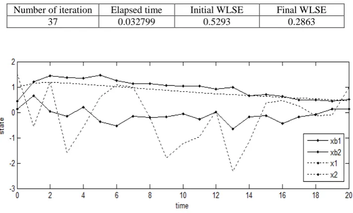
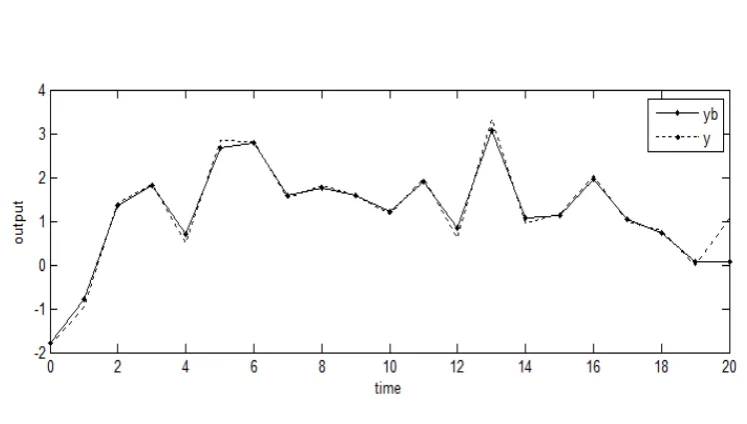
[image:10.595.128.484.447.662.2]

Table 1 shows the simulation result, where there is a 46 percent of the error reduction done by the algorithm proposed. Here, the final WLSE, which is 0.2863, is preferred since this value is smaller than the mean square error (MSE) of the EKF that is 0.4468. In Figure 1, the dynamics of the plant and state estimate are shown, where the state estimate tracks the plant dynamics slightly. In Figure 2, the behavior for the model output is similar equivalently to the original output, which shows the effectiveness of the algorithm proposed.

Table 1. Simulation Result

Number of iteration Elapsed time Initial WLSE Final WLSE 37 0.032799 0.5293 0.2863

Fig. 2. Output Trajectories

5

Concluding Remarks

The efficient computation approach for solving the nonlinear dynamic estimation problem was discussed in this paper. To solve this problem, the simplified linear model-based estimation problem with adding the adjusted parameters is introduced. During the computation procedure, the differences between the real system and the model used could be taken into account. The real output, which is measured from the real plant, is fed back into the model used in order to update the optimal solution of the model. This is done iteratively. As a result, the iterative solution converges to the true optimal solution of the original estimation problem despite model-reality differences when the convergence is achieved. For illustration, an example was studied and the results showed the efficiency of the algorithm proposed. In conclusion, the applicable of the algorithm proposed to nonlinear dynamic estimation problem is highly recommended.

References

1. Kalman, R. E.: A new approach to linear filtering and prediction problems. Journal of Basic Engineering. 35-45 (1960).

2. Kalman, R. E.: Contributions to the theory of optimal control. Bol. Soc. Mat. Mexicana. 102-119 (1960).

3. Kalman, R. E. and Bucy, R.S.: New results in linear filtering and prediction theory. Journal of Basic Engineering. 95-108 (1961).

[image:11.595.117.491.92.304.2]

5. Smith, G. L., Schmidt, S. F. and McGee, L. A.: Application of statistical filter theory to the optimal estimation of position and velocity on board a circumlunar vehicle. United States: National Aeronautics and Space Administration. (1962).

6. Ahmed, N. U.: Linear and Nonlinear Filtering for Scientists and Engineers. World Scientific Publishers, Singapore, New Jersey, London, Hong Kong. (1999).

7. Anderson, B. D. O. and More, J. B.: Optimal filtering. Englewood Cliffs NJ: Prentice-Hall. (1979). 8. Bagchi, A.: Optimal control of stochastic systems. New York: Prentice-Hall. (1993).

9. Julier S. and Uhlmann, J.: Unscented filtering and nonlinear estimation. Proceedings of the IEEE. 92, 401–422 (2004).

10.Uhlmann, J.: Dynamic map building and localization: new theoretical foundations. Ph.D. thesis, University of Oxford. (1995).

11.Julier, S. and Uhlmann, J.: A new method for the nonlinear transformation of means and covariances in nonlinear filters. IEEE Trans. on Automatic Control. 45, 477-482 (2000).

12.Rajamani, M. R.: Data-based techniques to improve state estimation in model predictive control. Ph.D. thesis, University of Wisconsin-Madison. (2007).

13.Olfati, S. R.: Collaborative target tracking using distributed Kalman filtering on mobile sensor networks. American Control Conference (ACC). 29 June-1 July, Dartmouth Coll., Hanover, NH, USA. 1100-1105 (2011).

14.Rigatos, G. G.: Derivative-free nonlinear Kalman filtering for MIMO dynamical systems: application to multi-DOF robotic manipulators. International Journal Advanced Robotic Systems. 8 (6), 47-61 (2011).

15.Krymskaya, M. V., Hanea, R. G. and Verlaan, M.: An iterative ensemble Kalman filter for reservoir engineering applications. Computational Geosciences. 13 (2), 235-244 (2009).

16.Andrea, F., Giovanni, S. and Claudio, C.: Enhanced accuracy of continuous glucose monitoring by online extended Kalman filtering. Diabetes Technology & Therapeutics. 12 (5), 353-363 (2010). 17.Feng, Z. G., Teo, K. L., Ahmed, N. U., Zhao, Y. and Yan, W. Y.: Optimal fusion of sensor data for

Kalman filtering. Discrete and Continuous Dynamical Systems–Series A. 14 (3), 483-503 (2006). 18.Kek, S. L., Teo K. L. and Mohd Ismail, A. A.: An integrated optimal control algorithm for

discrete-time nonlinear stochastic system. International Journal of Control. 83 (12), 2536-2545 (2010). 19.Kek, S. L., Teo, K. L. and Mohd Ismail, A. A.: Filtering solution of nonlinear stochastic optimal

control problem in discrete-time with model-reality differences. Numerical Algebra, Control and Optimization (NACO). 2 (1), 207-222 (2012).

20.Bryson, A. E. and Ho,Y. C.: Applied optimal control, Washington, DC: Hemisphere (1975).

21.Bar-Shalom, Y., Li, X. R and Kirubarajan, T.: Estimation with applications to tracking and navigation. New York: John Wiley & Sons, Inc (2001).

22.Lewis, F. L. and Syrmos, V. L.: Optimal Control, 2nd Ed., John Wiley & Sons (1995).

23.Simon, D.: Optimal state estimation: Kalman, H-infinity and nonlinear Approaches. John Wiley & Sons, Inc., Hoboken, New Jersey (2006).