Dynamic leveling control of a wireless self balancing rov using fuzzy logic controller

MOHAMMAD AFIF BIN AYOB

A thesis submitted in

fulfilment of the requirement for the award of the Masterof Electrical Engineering

Faculty of Electrical and Electronic Engineering UniversitiTun Hussein Onn Malaysia

ABSTRACT

ABSTRAK

Sebuahkenderaan yang dikendalikandarijauh (ROV) padaasasnyaadalah robot mudahalih yang beroperasi di dalam air yang dikawaldandikuasaiolehpengendalidi luarpersekitarankerja robot.Sepertimanakenderaanmarinyang lain, ROV direkauntukterapung di dalam air dimanajisimnyadisokongolehdayakeapungan yang disebabkanolehanjakan air olehstrukturkenderaan. Menyelaraskedudukan ROV

minisecaramenegakdalamresolusisentimeterdi dalamair

danmengekalkankeadaanitumemerlukantekniktersendirisebahagiannyakeranatekanan

dankeapungan yang dikenakanoleh air

kearahbadankenderaandansebahagiannyakeranagelombangrawak yang

dihasilkanoleh air itusendiri.Disebabkanhalini,

tujuanprojekiniadalahuntukmerekabentukdanmembangunkankeseimbangansendirike

apungansistemsebuah ROV mini

menggunakanpengawallogikkabur.Sebuahpenderiacecairtelahdigunakanuntukmembe rimaklumbalaskepadamikropengawal Arduino.Satuantaramukamesrapenggunagrafik

(GUI) telahdibangunkanuntukmemantaudata

secaramasasebenarsertamengawalkedudukanmenegakdaripada

ROV.Padaakhirprojek, sistemkawalankabur yang

dilaksanakanmenunjukkanprestasiyang

CONTENTS

ACKNOWLEDGEMENTS iv

ABSTRACT v

ABSTRAK vi

CONTENTS vii

LIST OF TABLES ix

LIST OF FIGURES x

LIST OF ABBREVIATIONS xii

LIST OF APPENDICES xiii

CHAPTER 1 INTRODUCTION 1

1.1 Report outline 1

1.2 Introduction 2

1.3 Problem statement 2

1.4 Aim and objectives 3

1.5 Scopes and limitations 3

CHAPTER 2 LITERATURE REVIEW 4

2.1 Introduction 4

2.2 Related work 4

2.3 Research comparison 11

CHAPTER 3 METHODOLOGY 13

3.1 Introduction 13

3.3 Hardware design 15

3.3.1 Mechanical 15

3.3.2 Electronics 17

3.3.2.1 Arduino Uno R3 mainboard 17 3.3.2.2 Liquid level sensor 18

3.3.2.3 Device connection 20

3.4 Software design 21

3.4.1 Wireless communication 21

3.4.2 Fuzzy logic controller 22

3.4.3 Graphical user interface (GUI) 25

CHAPTER 4 RESULTS AND ANALYSIS 27

4.1 Hardware development 27

4.1.1 Mechanical 27

4.1.2 Electronics 29

4.1.2.1 Micro pumps performance 29 4.1.2.2 Liquid level sensor 30

4.2 Software development 31

4.2.1 Fuzzy logic controller 31

4.2.2 Real-time response 35

CHAPTER 5 CONCLUSION AND RECOMMENDATION 39

5.1 Conclusion 39

5.2 Recommendation for future work 39

REFERENCES 41

LIST OF TABLES

TABLE TITLE PAGE

2.1 Comparison between each research 11

3.1 Arduino Uno R3 mainboard specification 17

3.2 Liquid level sensor specification 19

3.3 Fuzzy associative memory matrix (FAMM) 24

4.1 Flow rate capacity for micro pumps 29

4.2 ROV level consistency test 30

LIST OF FIGURES

FIGURE TITLE PAGE

2.1 ROV plant closed-loop system 5

2.2 ROV control strategy 6

2.3 Depth control simulation 6

2.4 Schematic diagram of a sperm whale’s head 7

2.5 VBS depth controller 8

2.6 VBS trim controller 8

2.7 VBS circuit diagram 9

2.8 ROV pneumatic control system 10

3.1 Flowchart of project activities 14

3.2 Device interfacing with Arduino Uno mainboard microcontroller

15

3.3 ROV prototype design 16

3.4 Arduino Uno R3 mainboard 17

3.5 eTape liquid level sensor 18

3.6 Typical output of liquid level sensor 19

3.7 Device connection diagramto Arduino Uno microcontroller board

20

3.8 Pairing two XBee modules in X-CTU 22

3.9 Components of fuzzy logic controller 23

3.10 Vertical positioning of a mini ROV control using fuzzy logic controller

24

4.1 ROV physical construction 28

4.2 Submerging ROV underwater 28

4.3 Simulated open loop controller for ROV leveling control system

31

4.4 A mini ROV open loop response 31

4.5 Fuzzy logic control block 32

4.6 Fuzzy logic control system response 32

4.7 Fuzzy logic control and PD control block 33

4.8 Fuzzy logic control and PID control block 33

4.9 Comparison of output response between fuzzy logic control and PD control system

34

4.10 Comparison of output response between fuzzy logic control and PID control system

34

4.11 ROV rising response from 0cm to 1cm 35

4.12 ROV sinking response from 1cm to 0cm 36

4.13 ROV sinking response from 1cm to -1cm 36

4.14 ROV rising response from 1cm to 2cm 37

LIST OF ABBREVIATIONS

AUV Autonomous Underwater Vehicle COG Center of Gravity

DC Direct Current

FAMM Fuzzy Associative Memory Matrix

GND Ground

GUI Graphical User Interface I/O Input/Output

ICSP In-Circuit Serial Programming LED light emitting diode

LQ-PID Least Squares Prediction Fuzzy Compensated PID LQR Linear Quadratic Regular

LSM Least Squares Method MISO Master In Slave Out MOSI Master Out Slave In

NM-FPID Normal Fuzzy Compensated PID PD Proportional Derivative

PID Proportional-Integral-Derivative PVC Polyvinyl Chloride

PWM Pulse Width Modulation

RF Radio Frequency

ROV Remotely Operated Vehicle

RST Reset

SCK Serial Clock

USB Universal Serial Bus

LIST OF APPENDICES

APPENDIX TITLE PAGE

A Arduino coding 44

CHAPTER 1

INTRODUCTION

1.1 Introduction

A remotely operated vehicle (ROV) is essentially an underwater mobile robot that is controlled and powered by an operator outside of the robot working environment via an umbilical cable or a remote control. A ROV differs from autonomous underwater vehicle (AUV) in a way that ROV always take command from its operator and takes no action autonomously. The boundless functionality of modern ROVs have brought great impact to the society from operations in both offshore and inshore by commercial, government, military and academic users [1].

1.2 Problem statement

ROV control presents several complications because of the nonlinearities model uncertainties and the influence of the external surroundings. Vertically positioning a mini ROV in centimeters resolution underwater and maintaining that state requires a distinctive technique. The reason is because of the pressure and buoyance force exerted by the water towards the vessel and also because of the random waves produced by the water itself. The study and design of a self-leveling control system for a mini ROV is significantly important because of numerous applications that can take benefits from it. Such examples include subsea installations, inspecting the hazardous inside of nuclear power plants, object location and recovery, and repairing complex deep water production systems.

1.3 Aim and objectives

The aim of the project is to design and develop a wireless self-leveling buoyancy system of a mini ROV by using fuzzy logic controller that has the ability for precise depth control. The objectives of this project on the other hand are as follows:

(i) To improve a remotely controlled mini ROV by using a microcontroller with feedback sensor.

(ii) To develop a self-balancing buoyancy system for a mini ROV based on a liquid level sensor.

(iii) To design the fuzzy controller for a self-leveling buoyancy system of a mini ROV.

(iv) To develop a wireless communication between a mini ROV and a computer. (v) To test the performance of the developed system in order to fulfill the

requirement.

1.4 Scopes and limitations

The scopes and limitations of the project are given below:

(iii) All communications with the mini ROV have been conducted wirelessly within the X-CTU and MATLAB graphical user interface (GUI).

(iv) The wireless system module was implemented by using XBee S2 1mW Wire Antenna with ZigBee 2.4GHz radio frequency (RF) protocol.

(v) The size of the mini ROV was less than 1m2 area and weighed less than 2kg. (vi) The mini ROV used non-submersible direct current (DC) controlled water

pump to vertically level its position.

(vii) The self-balancing system is based on the attached liquid level sensor that provided feedback to the fuzzy logic controller.

(viii) The testing of the mini ROV was done in calm and shallow water (<1m).

1.5 Report outline

The project in this report is divided into five chapters. The first chapter which is the project introduction represents the overview of the project that include the declaration of the problems, the objectives of the project, the limitations of the study, and the contributions to the research area.

Chapter 2 covers the review of each critical points of current knowledge including essential findings as well as theoretical and methodological contributions to a particular topic.

Chapter 3 explains the systematic study of methods that have been applied within the project that consists of project activities, system architecture, hardware design and software design.

Chapter 4 discusses and compares the data of results and analysis that has been obtained from the testing of hardware and software throughout the project development. The testing is divided into two parts; interface testing and system testing. The interface testing discusses all peripherals that are interfaced to the microcontroller while the system testing focuses on the high-level software operation.

CHAPTER 2

LITERATURE REVIEW

2.1 Introduction

In order to design and develop a dynamic leveling control of a wireless mini ROV, extensive research on buoyancy and depth control of the vehicle need to be fulfilled. This chapter will discuss previous studies that have been accomplished by other researchers in the same area. Comparison of the studies is given at the end of the discussion.

2.2 Related work

Folcher and Rendas [4] address the identification and the control of the vertical motion of the ROV Phantom 500. They split the matter in two decoupled problems: the propeller motion and the diving motion. The ROV can be controlled from the surface either manually by using joysticks or automatically by a surface computer. It is well equipped with a 3 axis compass, a depth (pressure) sensor, an altimeter, a sonar profiler, a video camera, and incremental encoders for the thrusters.

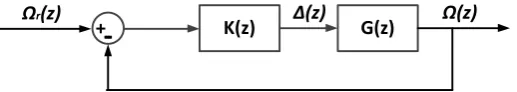
The controller generates the control signal Δ(n), as a function of the reference signal , and of the measured output . Equation 2.1 shows the controller in z-plane, where is the transfer function of the controller.

( ) (2.1)

The closed-loop block diagram of the plant is illustrated in Figure 2.1. In this figure, models the discrete time dynamics of the sample data system in series with a zero order hold. A major downside of the current system is that it relies on simplified decoupled models, and thus valid only under specific operating points (where some velocities and accelerations can be neglected).

K(z) Ωr(z)

+

_-

Figure 2.1: ROV plant closed-loop system

Tang and Luojun [5] developed a nonlinear depth control method for ROV. The method establishes the vertical motion model and uses least squares method (LSM) fitting multi-order output response of the control system. The fuzzy compensation is used to achieve overshoot suppression combined with proportional-integral-derivative (PID) controller. The LSM process the multi-order data fitting and generates the nonlinear predictor, where the predictor error is normalized as the input to the fuzzy controller.

PID

+

-Error E

Set D output

X

X

X

Fuzzy controller

Normalize

X

Sensor

-Predictor

Noise

+

Figure 2.2: ROV control strategy

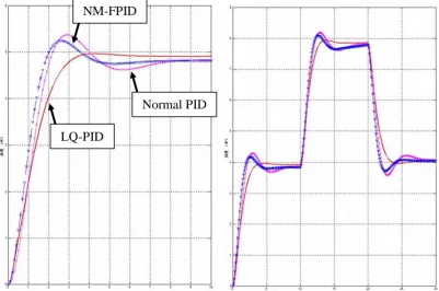
The comparison of simulation waveforms between normal fuzzy compensated PID (NM-FPID), normal PID controller, and the proposed least squares prediction fuzzy compensated PID (LQ-PID) is described in Figure 2.3. The simulation results show that the PID with prediction and fuzzy compensation control system response has a certain overshoot suppression performance and the system response speed faster than that of normal PID.

Figure 2.3: Depth control simulation Normal PID

NM-FPID

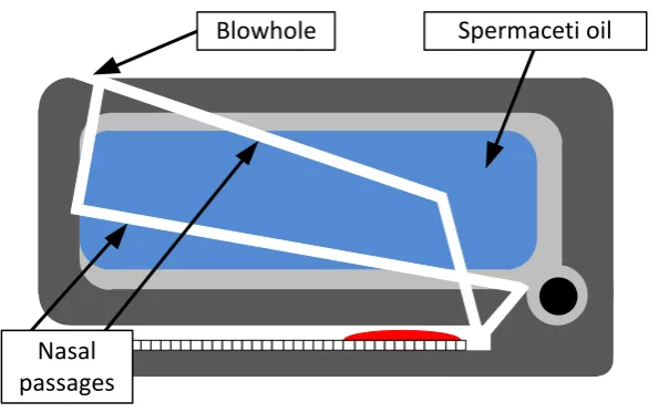
Shibuya, et al. [6] developed an underwater mobile robot with a buoyancy control system based on the spermaceti oil hypothesis originated back in 1970s [7]. The hypothesis insists that sperm whales melt and congeal their spermaceti oil that is located in their head and change the volume of the oil to control their own buoyancy. The anatomy of a sperm’s whale head is presented in Figure 2.4. The spermaceti organ that contains capillaries is located in the head. The nasal passage that goes around the organ acts as a coolant and heating element for the spermaceti oil. To choose the best materials as a spermaceti oil substitute, the densities of four materials at both liquid and solid states were measured. Afterwards, the buoyancy differences between both states were calculated. The experiment resulted in paraffin wax as the best substance.

Nasal passages

Blowhole Spermaceti oil

Figure 2.4: Schematic diagram of a sperm whale's head

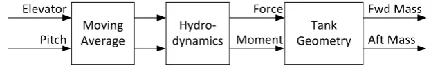
Tangirala and Dzielski [2] developed a variable buoyancy control system (VBS) for a large AUV to launch in shallow water (<10m) and to hover without propulsion. The vehicle is equipped with two VBS tank to meet these requirements. The resulting control problem is that the control variable (pump rate) is proportional to the third derivative of the sensed variable (depth). There are significant delays and forces are nonlinear (including discontinuous). The VBS control software operates in two modes: depth control mode as in Figure 2.5 and trim control mode as in Figure 2.6.

Depth

Command Quantizer

Derivative Wave Filter

Derivative Wave Filter Depth

Depth +

- Kp +- Kd +

-+1,0,-1

Figure 2.5: VBS depth controller

Moving Average

Hydro-dynamics

Tank Geometry Elevator

Pitch

Force

Moment

Fwd Mass

Aft Mass

Figure 2.6: VBS trim controller

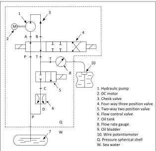
A long cruising range AUV equipped with a VBS system was developed by Zhao, et al. [8] and it was found that buoyancy is the resultant force between the AUV weight and the buoyancy of its displacement volume. The VBS of the long cruising range AUV was constructed with an oil tank, a rubber bladder which can regulate its displacement volume and a set of hydraulic drives system. The whole construction can bear the ambient sea water pressure when it works in 1000m depth.

The circuit diagram of the VBS for the AUV is shown in Figure 2.7. The displacement volume of the bladder is controlled by pumping the oil between the oil tank and the oil bladder with the hydraulic pump. This is to make the buoyancy of the AUV is altered without changing its weight. When the VBS computer receives the buoyancy adjustment command from the operator, it calculates the number of pump revolutions according to the ambient pressure of the AUV. It will then sends the pulse width modulation (PWM) signals to the driver of the DC motor.

M T T T T T T +

-

P T _T

D P 1 2 3 4 10 8 5 6 7 Q W

1. Hydraulic pump 2. DC motor 3. Check valve

4. Four-way three position valve 5. Two-way two position valve 6. Flow control valve 7. Oil tank

8. Flow rate gauge 9. Oil bladder

10. Wire potentiometer Q. Pressure spherical shell W. Sea water

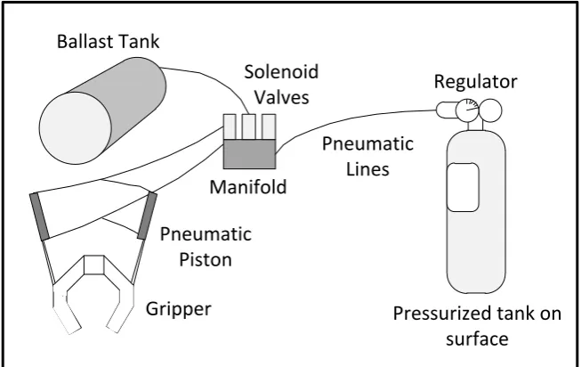
Wasserman, et al. [9] developed a dynamic buoyancy control of a tethered ROV using a variable ballast tank. The dynamic buoyancy control solution for the small-scale ROV is a pneumatic system that includes an air-filled ballast tank as depicted in Figure 2.8 with visual feedback from underwater cameras. The major parts of the system are the air source, the manifold and solenoids (used as the control system for the air), the pneumatic grippers, and the buoyancy control ballast tank. Plastic tubing is used as air lines between the major components.

The source of the air is a surface tank that is brought to the ROV through a single hose in ROV’s tether and is always pressurized. The ballast tank would be originally filled with water where a small hose would then expel the water from the tank and fill it with air to control its buoyancy.

Manifold

Regulator Ballast Tank

Pneumatic Piston

Gripper

Solenoid Valves

Pressurized tank on surface Pneumatic

Lines

2.3 Research comparison

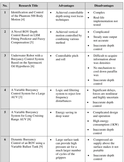
The comparisons for each of the previous studies regarding the buoyancy and depth control for ROV are summarized in Table 2.1.

Table 2.1: Comparison between each research

No. Research Title Advantages Disadvantages

1 Identification and Control of the Phantom 500 Body Motion [4]

 Achieved controllable depth using root locus techniques

 Complex

 Real-life

implementation not tested

2 A Novel ROV Depth Control Based on LSM Fitting Predictor and Fuzzy Compensation [5]

 Achieved vertical motion controlled by combining various method

 Complicated

 Steady state output not accurate

 Inaccurate depth control

3 Underwater Robot with a Buoyancy Control System Based on the Spermaceti Oil Hypothesis [6]

 Controllable pitch and roll

 Difficult to acquire information about wax densities

 No mechanism to cool down paraffin wax

 Inaccurate depth control

4 A Variable Buoyancy Control System for a Large AUV [3]

 Logic and filtering system to reject low frequency

disturbances

 Significant delays, forces are nonlinear and highly uncertain

 Inaccurate depth control

5 A Variable Buoyancy System for Long Cruising Range AUV [8]

 Energy saving in deep water

 Complicated design and operation

 High energy consumption (1KW)

 Inaccurate depth control

6 Dynamic Buoyancy Control of an ROV using a Variable Ballast Tank [9]

 Large surface tank can provide high pressure air for a much larger number of cycles of the grippers

 Compressed air supply above the surface makes it not portable

CHAPTER 3

METHODOLOGY

3.1 Introduction

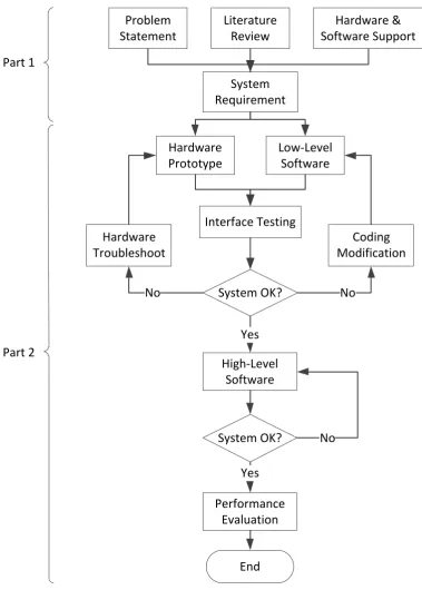
The project development of this study as shown in Figure 3.1 is divided into two parts namely Part 1 and Part 2. Each part represents the work to be done for Master Project 1 and Master Project 2 respectively. Part 1 starts by first identifying the problems that exist in the current system of a ROV. Extensive literature reviews has been done on related knowledge to assist in any ways that it may. Such reviews are based on international publications, engineering-related websites, and engineering books. Detail research in hardware is needed for the mini ROV electrical and electronic development in terms of availability, performance, and technical supports. The system requirement was then determined to proceed on this project.

Subsequently, if the overall system is working, high-level software that is the application to control the mini ROV movement and depth control is developed. Upon completing the system software, the overall system needs to be tested and analyzed to verify its functionality and performance.

Figure 3.1: Flowchart of project activities Problem

Statement

Literature Review

Hardware & Software Support

System Requirement

Hardware Prototype

Low-Level Software

Interface Testing

System OK? Hardware

Troubleshoot

Coding Modification

High-Level Software

No No

End System OK?

Performance Evaluation

Yes Yes

No Part 1

3.2 System architecture

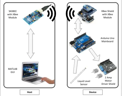
Figure 3.2 shows the interface between all devices that has been implemented to the mini ROV system by using master and slave setup. Controlling the mini ROV is done in a Windows GUI by a human operator with a personal computer. The computer is serially connected to the SKXBee board while simultaneously receive data and feedback from the onboard sensor of the mini ROV. Connection between master and slave control is made by using XBee series 2 wireless module. The module which is ZigBee compliant is chosen since it provides low transmission power rate and is suitable to use in short range data transmission [10].

SKXBEE with XBee

Module

MATLAB GUI

Arduino Uno Mainboard

Liquid Level Sensor

XBee Shield with XBee

Module

2 Amp Motor Driver Shield

Device Host

3.3 Hardware design

The hardware section gives further explanations on both mechanical and electronic parts. The mechanical part explains the prototype of the mini ROV design while the electronic part describes the interfacing between all of the electronic devices.

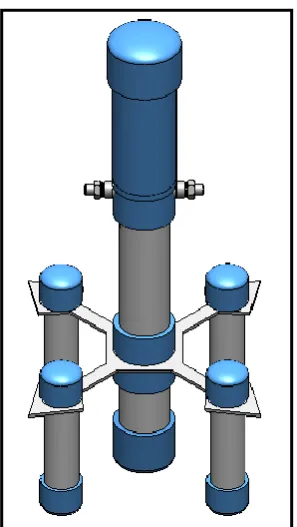
3.3.1 Mechanical

The mini ROV of this project was designed by using SolidWorks with every details and considerations taken into account. The prototype design is shown in Figure 3.3. The final version however had rather underwent some modifications and tweaks to cope with the overall system of this project.

Figure 3.3: Mini ROV prototype design

Since fluid pressure increases with depth and that the increased pressure exerted in all directions, thus there is an unbalanced upward force on the bottom of a submerged object [11]. To overcome this problem, four small cylindrical hulls are strategically placed around the main structure to further provide stability when the mini ROV is submerged into water. These hulls also help in increasing its positive buoyancy in order to compensate the weight of the mini ROV and can be manually adjusted for prototyping purpose.

The liquid level sensor is attached to the outside of the mini ROV. Archimedes principle stated that the buoyant force on a submerged object is equal to the weight of the fluid that is displaced on by the object [12]. In other words, when a solid body is partially or completely immersed in water, the apparent loss in weight will be equal to the weight of the displaced liquid. Since the amount of the displaced liquid is directly proportional to the height of the mini ROV being submerged, hence placing the sensor on the outside of the mini ROV is suitable and a fast way to properly determine its vertical position.

3.3.2 Electronics

3.3.2.1 Arduino Uno R3 mainboard

Figure 3.4: Arduino Uno R3 mainboard

Table 3.1: Arduino Uno R3 mainboard specification

Microcontroller ATmega328

Operating Voltage 5V

Input Voltage (recommended) 7-12V

Input Voltage (limits) 6-20V

Digital I/O Pins 14 (of which 6 provide PWM outputs)

Analog Input Pins 6

DC Current per I/O Pin 40mA

DC Current for 3.3V Pin 50mA

Clock Speed 16MHz

3.3.2.2 Liquid level sensor

Figure 3.5: eTape liquid level sensor

The sensor provides a resistive output that is inversely proportional to the level of the liquid, in which case when the liquid level is low, the output resistance will be high, and vice versa. The sensor has its own marking printed in centimeters and inches making it easier to manually monitor the fluid level. The specification of the sensor is given in Table 3.2. The sensor can be modeled as a variable resistor (300 - 1500Ω ±10%) and the typical output of the sensor is given in Figure 3.6 [14].

Table 3.2: Liquid level sensor specification

Sensor Length 10.1″ (257mm)

Active Sensor Length 8.4″ (213mm)

Resolution < 0.01″ (0.25mm)

Width 1.0″ (25.4mm)

Sensor Output 1500Ω empty, 300Ω full, ±10%

Temperature Range -9°C - 65°C

Resistance Gradient 140Ω/inch (56Ω/cm), ±10%

Figure 3.6: Typical output of liquid level sensor

To get the readings of the sensor when it is submerged, the following formula in Equation 3.1 is applied. The initial point at mark 15cm of the sensor has been chosen. The SensorValue is the current reading of the sensor in terms of resistance. The value 354 is the sensor reading at the initial point while the value 290 is the sensor reading 2cm above the initial point. The whole equation is multiplied by 2 since the range of the sensor calibration in this project is 2cm. The output of the equation will give the position of the sensor in centimeters resolution.

(3.1)

3.3.2.3 Device connection

A7

A4 A5 A6

ICSP TX

RX

GND Vin

RST 5V

GND

5V A0

M1+

M1-M2+

M2-Liquid Level Sensor

2 Amp Motor Driver Shield

XBee Shield with XBee Module

DC Pump 1

DC Pump 2

Figure 3.7: Device connection diagram to Arduino Uno microcontroller board

The liquid level sensor uses 5V, GND, and analog A0 port from Arduino. The XBee shield that is attached with the XBee module is connected to the microcontroller via the in-circuit serial programming (ICSP) header. The XBee module works as a transceiver; therefore it transmits and receives data via the TX and RX pin. The ICSP header of the Arduino consists of a Master In Slave Out (MISO), Master Out Slave In (MOSI), Serial Clock (SCK), +5V, ground, and reset pin. Similar to the motor shield, it can be stacked right on top of the board while still having all required pins connected.

3.4 Software design

The software section gives explanations regarding the wireless communication setup between the Arduino microcontroller and computer. Other details include fuzzy logic control that is used in this project and the GUI for the control and data monitoring of the mini ROV.

3.4.1 Wireless communication

Every XBee modules have their own unique addresses. In order to get the wireless communication to work, both of the source and destination address of the XBee modules need to be paired with each other. There are two ways to do the setup; one by using a small list of programming code while another is simply by using the X-CTU software provided by Digi International. X-X-CTU is a free software that not only can be used to set the communication parameters on the XBee but also a monitoring platform to transmit and receive data communications.

F

igure

3.

8

:

P

airing t

wo X

B

ee

modul

es in X

-C

T

The destination address high and low for each module needs to be the exact address as the source address high and low for the other module. This can be done by simply copy the value of the source address from one module and paste it to the destination address of the other module. The same method applied for both XBee modules.

3.4.2 Fuzzy logic controller

There are various controller design theories that can be used to maintain the leveling control of the mini ROV system such as fuzzy logic controller, PID controller, adaptive controller, pole placement, linear quadratic regular (LQR), and robust control. In this study, fuzzy logic controller is used to control the vertical motion of the mini ROV. The components of fuzzy logic controller are shown in Figure 3.9. It generally comprises of four principal modules; fuzzifier, knowledge base, inference engine, and defuzzifier.

Fuzzifier

Inference

Defuzzifier

Engine

Knowledge

Base

Fuzzy Controller

Process

state

Crisp control signal

REFERENCES

1. Marine Technology Society (2010). ROV Applications – What ROVs Can Do. Retrieved on April 5, 2012, from http://www.rov.org/rov_applications .cfm

2. Psarros, D., Papadimitriou, V., and Chatzakos, P., A service robot for subsea flexible risers, IEEE Robotics & Automation Magazine, 2010, Vol. 7, pp. 55-63. Retrieved July 17, 2012, from IEEE database.

3. Tangirala, S. and Dzielski, J. “A Variable Buoyancy Control System for a Large AUV,” IEEE Journal of Oceanic Engineering, Vol. 32, No. 4, 2007, pp. 762-771. doi: 10.1109/JOE.2007.911596.

4. Folcher, J. P. and Rendas, M. J. "Identification and Control of the Phantom 500 Body Motion," MTS/IEEE Conference and Exhibition of OCEANS 2001, Honolulu, 5-8 November 2001, pp.529-535.

5. Tang, Z. and Luojun, P. Y., “A Novel ROV Depth Control Based on LSM Fitting Predictor and Fuzzy Compensation,” 3rd International Conference on Advanced Computer Theory and Engineering (ICACTE), 2010, Chengdu, 20-22 August 2010, V2-612 - V2-614.

6. Shibuya, K, Kado, Y., Honda, S., Iwamoto, T. and Tsutsumim, K., “Underwater Robot with a Buoyancy Control System Based on the Spermaceti Oil Hypothesis,” Proceedings of the 2006 IEEE/RSJ Interational Conference on Intelligent Robots and Systems, Beijing, 9-15 October 2006, pp. 3012-3017.

7. Clarke, M. R. “Buoyancy Control as a Function of the Spermaceti Organ in the Sperm Whale,” Journal of the Marine Biological Association of the

United Kingdom, Vol. 58, Issue 1, 1978, pp. 27-71. doi:

8. Zhao, W., Xu, J., and Zhang, M., “A Variable Buoyancy System for Long Cruising Range AUV,” 2010 International Conference on Computer, Mechatronics, Control and Electronic Engineering (CMCE), Harbin, 24-26 August 2010, pp.585-588.

9. Wasserman, K. S., Mathieu, J. L., Wolf, M. I., Hathi, A., Fried, S. E. and Baker, A. K., “Dynamic Buoyancy Control of an ROV using Variable Ballast Tank,” Proceedings of OCEANS 2003, Massachusetts, 22-26 September 2003, pp. 2888-2893.

10. MaxStream, (2007). XBee Series 2 OEM RF Modules. Retrieved May 14, 2012, from p. 4 at ftp://ftp1.digi.com/support/documentation/90000866_A .pdf

11. Nave, R. (1998), Pressure. Retrieved on May 24, 2012, from http://hyperphysics.phy-astr.gsu.edu/hbase/pbuoy.html

12. Carrol, B. (2009), Archimedes Principle. Retrieved on May 24, 2012, from http://physics.weber.edu/carroll/archimedes/principle.htm

13. Arduino, (2012), Arduino Uno. Retrieved on May 26, 2012, from http://arduino.cc/en/Main/ArduinoBoardUno

14. Milone Technologies, (2012), eTape Specification. Retrieved on May 26, 2012, from p. 1 at http://www.milonetech.com/uploads/eTape_Datasheet_ 12110215TC-8.pdf

15. Xu, M., “Adaptive Fuzzy Logic Depth Controller for Variable Buoyancy System of Autonomous Underwater Vehicles,” Proceedings of the Third IEEE Conference on Fuzzy Systems, Florida, 26-29 June 1994, pp. 1191-1196.

VITA

LIST OF PUBLICATIONS

1. Ayob, M. A., Hanafi, D., Johari, A., Dynamic leveling control of a wireless self-balancing ROV using fuzzy logic controller, in SCIRP Intelligent Control and Automation (ICA 2012), 2012. (submitted)

Arduino coding

1 int RiseMotorSpeed = 5; //pwm //motor 1 2 int SinkMotorSpeed = 6; //pwm //motor 2 3 int RiseMotorEn = 4; //enable pin 4 int SinkMotorEn = 7; //enable pin 5

6 int LED = 13; 7

8 float x[3], input[2], sensor, sensorValue;

9 float fsE[2], sectorE[2], fsDE[2], sectorDE[2], centerout[2]; 10

11 float Mfout1, Mfout2; 12

13

14 //*******************************************************************// 15 //Declaration of Fuzzy Set for Input 1 (Error) // 16 //*******************************************************************// 17

18 19 float

20 a1 = 0, b1 = -1, c1 = -0.5, 21 a2 = -1, b2 = -0.5, c2 = 0, 22 a3 = -0.5, b3 = 0, c3 = 0.5, 23 a4 = 0, b4 = 0.5, c4 = 1, 24 a5 = 0.5, b5 = 1, c5 = 0; 25

26 //F=[a1 b1 c1;a2 b2 c2;a3 b3 c3;a4 b4 c4;a5 b5 c5;]; 27

28

29 //*******************************************************************// 30 //Declaration of Fuzzy Set for Input 2 (DeltaError) // 31 //*******************************************************************// 32

33 34 float

35 a6 = 0, b6 = -1, c6 = -0.375, 36 a7 = -0.75, b7 = -0.375, c7 = 0, 37 a8 = -0.375, b8 = 0, c8 = 0.375, 38 a9 = 0, b9 = 0.375, c9 = 0.75, 39 a10 = 0.375, b10 = 1, c10 = 0; 40

41 //G=[a6 b6 c6;a7 b7 c7;a8 b8 c8;a9 b9 c9;a10 b10 c10;]; 42

43

44 //*******************************************************************// 45 //Rules Designation (25 Rules) // 46 //*******************************************************************// 47

48

49 float co1[5] = { -1.0, -0.5, -1.0, -0.5, -1.0 }; 50 float co2[5] = { -1.0, -0.5, -0.3, -0.5, -1.0 }; 51 float co3[5] = { +0.0, +0.0, +0.0, +0.0, +0.0 }; 52 float co4[5] = { +1.0, +0.5, +0.3, +0.5, +1.0 }; 53 float co5[5] = { +1.0, +0.5, +1.0, +0.5, +1.0 }; 54

55 56 57 58

59 // the setup routine runs once the reset button is pressed: 60 void setup() {

61 // initialize serial communication at 9600 bits per second: 62 Serial.begin(9600);

63 pinMode(RiseMotorEn, OUTPUT); 64 pinMode(SinkMotorEn, OUTPUT); 65 digitalWrite(RiseMotorEn, HIGH); 66 digitalWrite(SinkMotorEn, HIGH); 67

71 input[0] = 0; 72 input[1] = 0; 73 x[2] = 0; 74 }

75 76 77

78 // the loop routine runs over and over again forever: 79 void loop() {

80

81 //*******************************************************************// 82 //Declaration of Fuzzy Set for Input 1 (Error) (INPUT) // 83 //*******************************************************************// 84

85

86 for (int L=0; L<=5; L++) { //delay 1s 87 digitalWrite(LED, LOW);

88 delay(200);

89 digitalWrite(LED, HIGH); 90 delay(200);

91 } 92

93 sensorValue = analogRead(A0);

94 //sensor = ((512-sensorValue)/(512-1023)); // test with POT 95 sensor = ((334-sensorValue)/(334-300))*2; // LLV. 0 = 15cm 96

97 //delay(3000);

98 if (!Serial.available()); { // wait until there is signal send from computer 99 input[0] = Serial.read();

100 }

101 if (input[0] == 45) { // read -ve input. -ve == 45 102 while (!Serial.available());

103 input[0] = Serial.read();

104 input[0] = -(((input[0]-48)/2)*1.75); 105 input[1] = input[0];

106 } 107

108 else if (input[0] > 45) { // read +ve input 109 input[0] = ((input[0]-48)/2)*1.75;

110 input[1] = input[0]; 111 }

112 113 114 else {

115 input[0] = input[1]; 116 }

117 118 119

120 x[0] = input[0] - sensor; // error

121 x[1] = x[0] - x[2]; // delta error = new error - old error 122 x[2] = x[0]; // old error

123

124 Serial.println(sensor); 125

126

127 //Region a

128 if (x[0] <= b1) { 129 fsE[0] = 1; 130 fsE[1] = 1;

131 sectorE[0] = -2; //NB 132 sectorE[1] = -2; //NB 133 }

134

135 //Region b

136 else if (x[0] > b1 && x[0] <= b2) { 137 fsE[0] = (c1-x[0])/(c1-b1); 138 fsE[1] = (x[0]-a2)/(b2-a2); 139 sectorE[0] = -2; //NB 140 sectorE[1] = -1; //N 141 }

142

143 //Region c

147 sectorE[0] = -1; //N 148 sectorE[1] = 0; //Z 149 }

150

151 //Region d

152 else if (x[0] > b3 && x[0] <= b4) { 153 fsE[0] = (c3-x[0])/(c3-b3); 154 fsE[1] = (x[0]-a4)/(b4-a4); 155 sectorE[0] = 0; //Z 156 sectorE[1] = 1; //P 157 }

158

159 //Region e

160 else if (x[0] > b4 && x[0] <= b5) { 161 fsE[0] = (c4-x[0])/(c4-b4); 162 fsE[1] = (x[0]-a5)/(b5-a5); 163 sectorE[0] = 1; //P 164 sectorE[1] = 2; //PB 165 }

166

167 //Region f

168 else if (x[0] > b5) { 169 //else {

170 fsE[0] = 1; 171 fsE[1] = 1;

172 sectorE[0] = 2; //PB 173 sectorE[1] = 2; //PB 174 }

175 176

177 //*******************************************************************// 178 //Declaration of Fuzzy Set for Input 2 (Delta Error) // 179 //*******************************************************************// 180

181

182 //Region a: 183 if (x[1] <= b6) { 184 fsDE[0] = 1; 185 fsDE[1] = 1;

186 sectorDE[0] = -2; //NB 187 sectorDE[1] = -2; //NB 188 }

189

190 //Region b:

191 else if (x[1] > b6 && x[1] <= b7) { 192 fsDE[0] = (c6-x[1])/(c6-b6); 193 fsDE[1] = (x[1]-a7)/(b7-a7); 194 sectorDE[0] = -2; //NB 195 sectorDE[1] = -1; //N 196 }

197

198 //Region c:

199 else if (x[1] > b7 && x[1] <= b8) { 200 fsDE[0] = (c7-x[1])/(c7-b7); 201 fsDE[1] = (x[1]-a8)/(b8-a8); 202 sectorDE[0] = -1; //N 203 sectorDE[1] = -0; //Z 204 }

205

206 //Region d:

207 else if (x[1] > b8 && x[1] <= b9) { 208 fsDE[0] = (c8-x[1])/(c8-b8); 209 fsDE[1] =( x[1]-a9)/(b9-a9); 210 sectorDE[0] = 0; //Z

211 sectorDE[1] = 1; //P 212 }

213

214 //Region e:

215 else if (x[1] > b9 && x[1] <= b10) { 216 fsDE[0] = (c9-x[1])/(c9-b9); 217 fsDE[1] = (x[1]-a10)/(b10-a10); 218 sectorDE[0] = 1; //P

219 sectorDE[1] = 2; //PB 220 }

221

223 //else { 224 fsDE[0] = 1; 225 fsDE[1] = 1;

226 sectorDE[0] = 2; //NB 227 sectorDE[1] = 2; 228 }

229 230

231 //*******************************************************************// 232 //Fuzzy Inference System (MAMDANI METHOD) // 233 //*******************************************************************// 234

235

236 if (fsE[0] < fsDE[0]) { //take min 237 Mfout1 = fsE[0];

238 } 239 else

240 Mfout1 = fsDE[0]; 241

242

243 if (fsE[1] < fsDE[1]) { //take min 244 Mfout2 = fsE[1];

245 } 246 else

247 Mfout2 = fsDE[1]; 248

249 250

251 //*******************************************************************// 252 //Rules Designation (25 Rules) // 253 //*******************************************************************// 254

255 //**************************************Row-1 256

257 int k;

258 for (k = 0; k < 2; k++) {

259 if (sectorE[k] == -2 && sectorDE[k] == -2) { 260 centerout[k] = co1[0];

261 }//co = central output 262

263 else if (sectorE[k] == -2 && sectorDE[k] == -1) { 264 centerout[k] = co1[1];

265 } 266

267 else if (sectorE[k] == -2 && sectorDE[k] == 0) { 268 centerout[k] = co1[2];

269 } 270

271 else if (sectorE[k] == -2 && sectorDE[k] == 1) { 272 centerout[k] = co1[3];

273 } 274

275 else if (sectorE[k] == -2 && sectorDE[k] == 2) { 276 centerout[k] = co1[4];

277 } 278

279 //**************************************Row-2 280

281 else if (sectorE[k] == -1 && sectorDE[k] == -2) { 282 centerout[k] = co2[0];

283 } 284

285 else if (sectorE[k] == -1 && sectorDE[k] == -1) { 286 centerout[k] = co2[1];

287 } 288

289 else if (sectorE[k] == -1 && sectorDE[k] == 0) { 290 centerout[k] = co2[2];

291 } 292

293 else if (sectorE[k] == -1 && sectorDE[k] == 1) { 294 centerout[k] = co2[3];

295 } 296

299 } 300

301 // ************************************Row-3 302

303 else if (sectorE[k] == 0 && sectorDE[k] == -2) { 304 centerout[k] =co3[0];

305 } 306

307 else if (sectorE[k] == 0 && sectorDE[k] == -1) { 308 centerout[k] = co3[1];

309 } 310

311 else if (sectorE[k] == 0 && sectorDE[k] == 0) { 312 centerout[k] = co3[2];

313 } 314

315 else if (sectorE[k] == 0 && sectorDE[k] == 1) { 316 centerout[k] = co3[3];

317 } 318

319 else if (sectorE[k] == 0 && sectorDE[k] == 2) { 320 centerout[k] = co3[4];

321 } 322

323 //*****************************************Row-4 324

325 else if (sectorE[k] == 1 && sectorDE[k] == -2) { 326 centerout[k] = co4[0];

327 } 328

329 else if (sectorE[k] == 1 && sectorDE[k] == -1) { 330 centerout[k] = co4[1];

331 } 332

333 else if (sectorE[k] == 1 && sectorDE[k] == 0) { 334 centerout[k] = co4[2];

335 } 336

337 else if (sectorE[k] == 1 && sectorDE[k] == 1) { 338 centerout[k] = co4[3];

339 } 340

341 else if (sectorE[k] == 1 && sectorDE[k] == 2) { 342 centerout[k] = co4[4];

343 } 344

345 ////***************************************Row-5 346

347 else if (sectorE[k] == 2 && sectorDE[k] == -2) { 348 centerout[k] = co5[0];

349 } 350

351 else if (sectorE[k] == 2 && sectorDE[k] == -1) { 352 centerout[k] = co5[1];

353 } 354

355 else if (sectorE[k] == 2 && sectorDE[k] == 0) { 356 centerout[k] = co5[2];

357 } 358

359 else if (sectorE[k] == 2 && sectorDE[k] == 1) { 360 centerout[k] = co5[3];

361 } 362

363 else if (sectorE[k] == 2 && sectorDE[k] == 2) { 364 //else {

365 centerout[k] = co5[4]; 366 }

367 368 } 369

370 ////*********************************************************// 371 ////Defuzzification Using Centroid of Gravity Method

372 ////*********************************************************// 373

375 376

377 if (COG > 0) {

378 digitalWrite(RiseMotorEn, HIGH); // motor 1 379 analogWrite(RiseMotorSpeed, 255);

380 for (int r=0; r<=30; r++) {

381 delay(COG*500); //40s = 1cm 382 sensorValue = analogRead(A0);

383 sensor = ((334-sensorValue)/(334-300))*2; // LLV. 0 = 15cm // LLV. 0 = 15cm 384 Serial.println(sensor);

385 }

386 analogWrite(RiseMotorSpeed, 0); 387 }

388

389 else if (COG < 0) {

390 digitalWrite(SinkMotorEn, HIGH); // motor 2 391 analogWrite(SinkMotorSpeed, 255);

392 for (int s=0; s<=30; s++) { //s<=34

393 delay(-(COG*500)); //16.67s = 1cm 394 sensorValue = analogRead(A0);

395 sensor = ((334-sensorValue)/(334-300))*2; // LLV. 0 = 15cm // LLV. 0 = 15cm 396 Serial.println(sensor);

397 }

398 analogWrite(SinkMotorSpeed, 0); 399 }

400 else if (COG == 0) {

401 analogWrite(SinkMotorSpeed, 0); 402 analogWrite(RiseMotorSpeed, 0); 403 }

MATLAB GUI coding

function varargout = gui2(varargin)

% Begin initialization code - DO NOT EDIT gui_Singleton = 1;

gui_State = struct('gui_Name', mfilename, ... 'gui_Singleton', gui_Singleton, ... 'gui_OpeningFcn', @gui2_OpeningFcn, ... 'gui_OutputFcn', @gui2_OutputFcn, ... 'gui_LayoutFcn', [] , ...

'gui_Callback', []); if nargin && ischar(varargin{1})

gui_State.gui_Callback = str2func(varargin{1}); end

if nargout

[varargout{1:nargout}] = gui_mainfcn(gui_State, varargin{:}); else

gui_mainfcn(gui_State, varargin{:}); end

% End initialization code - DO NOT EDIT

% --- Executes just before gui2 is made visible.

function gui2_OpeningFcn(hObject, eventdata, handles, varargin) % This function has no output args, see OutputFcn.

% hObject handle to figure

% eventdata reserved - to be defined in a future version of MATLAB % handles structure with handles and user data (see GUIDATA) % varargin command line arguments to gui2 (see VARARGIN)

axis off

backgroundImage = importdata('uthm.jpg'); %select the axes

axes(handles.logo); %place image onto the axes image(backgroundImage); %remove the axis tick marks axis off

% Choose default command line output for GUI handles.output = hObject;

% Update handles structure guidata(hObject, handles);

% UIWAIT makes gui2 wait for user response (see UIRESUME) % uiwait(handles.figure1);

clc; clear all; clear s; global s;

s = serial('COM3');

% --- Outputs from this function are returned to the command line. function varargout = gui2_OutputFcn(hObject, eventdata, handles) % varargout cell array for returning output args (see VARARGOUT); % hObject handle to figure

% eventdata reserved - to be defined in a future version of MATLAB % handles structure with handles and user data (see GUIDATA)

% Get default command line output from handles structure varargout{1} = handles.output;

% --- Executes on button press in start.

function start_Callback(hObject, eventdata, handles) % hObject handle to start (see GCBO)

global s;

TimeInterval=0.01; loop=500;

time = now; ori = now; sensor = 90;

handles.plot = plot(handles.graph,time,sensor,'LineWidth',2,'Color',[1 1 1]); sensor(1)=90;

time(1)=0; count = 1; fopen(s);

while ~isequal(count,loop)

sensor(count) = fscanf(s,'%f');

set(handles.present, 'String', sensor(count)); time(count) = (now-ori)*100000;

%axes(handles.axes2)

set(handles.plot,'YData',sensor,'XData',time); set(handles.graph, 'YGrid','on',...

'YColor',[0.043 0.518 0.78],... 'XGrid','on',...

'XColor',[0.043 0.518 0.78],... 'Color',[0 0 0]);

pause(TimeInterval); count = count +1; end

fclose(s); delete(s); clear s;

function desired_Callback(hObject, eventdata, handles) % hObject handle to desired (see GCBO)

% eventdata reserved - to be defined in a future version of MATLAB % handles structure with handles and user data (see GUIDATA)

global s; time = now;

a=get(hObject,'String'); a=char(a);

fprintf(s,'%s',a);

% --- Executes during object creation, after setting all properties. function desired_CreateFcn(hObject, eventdata, handles)

% hObject handle to desired (see GCBO)

% eventdata reserved - to be defined in a future version of MATLAB

% handles empty - handles not created until after all CreateFcns called

% See ISPC and COMPUTER.

if ispc && isequal(get(hObject,'BackgroundColor'), get(0,'defaultUicontrolBackgroundColor'))