BIROn - Birkbeck Institutional Research Online
Chandna, Swati and Wang, W. (2018) Bootstrap averaging for model-based
source separation in reverberant conditions.
IEEE/ACM Transactions on
Audio, Speech and Language Processing 26 (4), pp. 806-819. ISSN
2329-9290.
Downloaded from:
Usage Guidelines:
Please refer to usage guidelines at
or alternatively
Bootstrap Averaging for Model-Based Source
Separation in Reverberant Conditions
Swati Chandna and Wenwu Wang,
Senior Member, IEEE
Abstract—Recently proposed model-based methods use time-frequency (T-F) masking for source separation, where the T-F masks are derived from various cues described by a frequency domain Gaussian Mixture Model (GMM). These methods work well for separating mixtures recorded in low-to-medium level of reverberation, however, their performance degrades as the level of reverberation is increased. We note that the relatively poor performance of these methods under reverberant conditions can be attributed to the high variance of the frequency-dependent GMM parameter estimates. To address this limitation, a novel bootstrap-based approach is proposed to improve the accuracy of expectation maximization (EM) estimates of a frequency-dependent GMM based on an a priori chosen initialization scheme. It is shown how the proposed technique allows us to construct time-frequency masks which lead to improved model-based source separation for reverberant speech mixtures. Experiments and analysis are performed on speech mixtures formed using real room-recorded impulse responses.
Index Terms—Gaussian mixture model, EM algorithm, boot-strap averaging, model-based source separation, time-frequency masking, reverberant speech mixtures, audio signal processing, spectral histogram
I. INTRODUCTION
S
Ource separation is defined as the problem of separating multiple sources mixed through an unknown mixing sys-tem (channel), using only the syssys-tem outputs (e.g. observed mixtures of speech). LetI denote the number of sources and M denote the number of channels. At discrete time point n∈ {1, . . . , N}, the system outputxm(n)at themth channelis a convolutive mixture of the form
xm(n) = I ∑
i=1
si(n)∗him(n)∗em(n), (1)
where∗ denotes convolution,si(n)is theith source,him(n)
for m = 1, . . . , M, is the room impulse response from source ito channel m, andem(n)denotes convolutive noise.
The choice of a convolutive noise is made for analytical convenience as it leads to an additive term in the log-magnitude and phase domains, [1]. For each i = 1, . . . , I, let si = [si(1), . . . , si(N)]T denote the source observed
at N time points, and similarly, for each m = 1, . . . , M,
S. Chandna is with the Dept. of Economics, Mathematics and Statis-tics at Birkbeck, University of London, London WC1E 7HX, UK (email: [email protected]) and W. Wang is with the Centre for Vision, Speech and Signal Processing (CVSSP), Department of Electrical and Electronic Engineering, University of Surrey, Guildford GU2 7XH, UK (e-mail: [email protected])
let xm = [xm(1), . . . , xm(N)]T denote the corresponding
mixture vector. Then the problem of source separation deals with the estimation of the source vectorss1, . . . ,sI, given the
mixture vectorsx1, . . . ,xM. This problem is termed
underde-termined when the number of observed mixtures, M, is less than the number of sources,I, that comprise the mixture.
In many real-world applications, the population may consist of several sub-populations and a standard distribution is not able to capture the variation over these sub-populations effec-tively. Finite mixture1models, as the name suggests, are exten-sively used to model such data with a finite mixture of standard distributions. Mixture distributions are extremely popular in areas such as audio-signal processing, image analysis, and geology, where they are used to model spectrograms in the time-frequency domain. Here, the time-frequency analysis of piecewise stationary signals allows the use of GMMs over time frames at each frequency. We shall refer to such frequency-specific GMMs as frequency domain GMMs. Some examples of applications employing GMMs in the frequency domain are [2], [3], [4] in speech signal analysis; [5], [6] in image analysis.
Model-based blind source separation for exactly determined and underdetermined speech mixtures such as [1], [7], [8], [9], are more recent examples of applications in speech analysis involving frequency-specific GMMs. These methods have gained significant popularity due to their simple model-based approach for integration of cues. In these methods, a by-product of the EM algorithm, used to estimate parameters of the frequency domain GMM, is a time-frequency (T-F) mask that allows separation of the target source of interest from the source of interference. These methods perform extremely well for mixtures recorded under low-to-medium levels of reverberation, however, their performance degrades as the reverberation level is increased. The poor performance of such algorithms for reverberant mixtures is attributed to inaccurate EM estimation of the frequency-dependent GMM parameters. More generally, this is due to the absence of an explicit model for reverberation. In addition to this, the frequency domain GMM in these algorithms, [1], [7], [8], relies on the assumption of the cues being independent. As noted in [8, sec. III.A], this assumption of the cues being independent does not hold in practice and is used as a convenient way to make the problem of source separation tractable. Overall, this results in a misspecified mixture model, leading to EM estimates with a very high variance. We show how better EM estimates of the target source parameters can be obtained using
1Note that the term ‘mixture’ here refers to a mixture of distributions and
the proposed bootstrap-based procedure to improve model-based source separation from reverberant speech mixtures. Our method is described for a univariate GMM in the frequency domain. Note that this does not require the observed time domain sample to be univariate, for example, as in the source separation algorithm of [1], where a univariate frequency do-main GMM is constructed by transforming a two-dimensional vector observation of speech mixtures.
Bootstrap methods are commonly used to draw inference on statistics of interest when no theoretical results are available, or when inference based on theoretical results is computationally intractable, such as to obtain standard errors and confidence intervals, [10]. Non-traditional applications of bootstrap which show how it can also facilitate a more robust statistical analysis are found, e.g., in machine learning to improve the forecast accuracy of models selected by unstable decision rules, [11], as well as in the area of pattern analysis where it is applied to the problem of fitting ellipse segments to noisy data to eliminate bias in the ellipse estimates [12]. The use of bootstrap for EM estimates of a frequency-dependent GMM, or to improve source separation performance as shown in our work, to the best of our knowledge, has never been mentioned in the literature and is the contribution of this paper. We would like to point out that the proposed idea of bootstrap averaging is very well-suited to the above mentioned source separation problem since the GMM appears in the frequency domain, and hence can be bootstrapped indirectly using the sample in the time domain, details of which are provided in this paper. Results from a set of preliminary experiments using this approach were presented in [13].
More recently, there has been a growing interest in tech-niques employing non-negative matrix factorization (NMF) and deep neural networks (DNN) to the problem of source separation. The idea with NMF for multichannel source sep-aration, e.g. [14], is to model the power spectrogram of each source in the T-F domain as a product of two non-negative matrices. Then modeling the short-time-Fourier transform (STFT) of each source as the sum of a finite number of latent Gaussian components, an EM implementation and a multiplicative update (MU) approach have been proposed to estimate the matrix factors (determining the variance of the Gaussian components) as well as the unknown convolutive mixing matrix. An NMF and spatial covariance model has also been studied for underdetermined source separation under reverberant conditions [15]. This is based on the EM algorithm for estimation of the model parameters and the authors note the sensitivity of their estimates to parameter initialization as well as degrading performance with increasing reverberation times. Another formulation for multichannel NMF described in [16], clusters the NMF bases according to their spatial properties. DNNs have been used to separate sources from binaural mixtures under reverberation via a binary classification, e.g. [17] and related work by [18], or using a probabilistic time-frequency mask, e.g. [19]. The latter approach integrates binaural cues following the model-based method of [8]. A multichannel source separation method is described in [20].
DNN based approaches are supervised methods that need training data sets, which may not always be available.
Model-based approaches such as [1], [9], [8] considered in this paper as well as NMF methods for source separation allow the inclusion of spatial and spectral cues; do not require training data and are easier to deploy in unfamiliar environments. Noting these points, it is of interest to study improvements that can be achieved with such model-based methods and are the subject of this paper. Our approach is illustrated using the method of [8] and can also be adapted, for example, to improve the NMF-based multichannel source separation of [14], as discussed in section VIII.
A. Contributions and organization
Following some background and notation on GMMs and their EM estimation, the contributions of this paper are pre-sented as follows:
1) The proposed idea of bootstrap averaging is described in section III. A simulation example to illustrate the case of sub-optimal EM estimates and the use of averaging to reduce the mean-squared-error is discussed. This experi-ment shows the benchmark improveexperi-ment (measured via MSE) that may be achieved via the proposed method in an ideal set-up (without bootstrapping).
2) Model-based source separation focusing on the forms of frequency domain GMMs that appear in such applications is described in section IV.
3) Bootstrap averaging for the source separation algorithm of [8] is presented in section V. Simulation experiments using speech mixtures formed with real room-recorded impulse responses are included in section VI.
4) A further in-depth analysis to understand overall improve-ments in model-based source separation via the proposed methodology is provided in section VII.
II. BACKGROUND ANDNOTATION
Let G ≡ {gY|j(y|λj), j = 1, . . . , d} denote a set of
d probability density functions, each with parameter vector
λ1, . . . ,λd, respectively. Let y1, . . . , yK denote a length-K
sample from a scalar-valued random processY, such that each observation of the length-K sample arises from one of the d density functions inG. Forj= 1, . . . , d, letZj(y)denote an
indicator variable which takes the value one if observation y comes from thejth component density gY|j(y|λj). Consider
the case where Zj(y) is not observed for y ≡ y1, . . . , yK,
i.e., the membership of yi for i = 1, . . . , K in one of the d
components is unknown. Then, the probability density function ofY, denoted asgY(.)is obtained by marginalizing the joint
density ofY andZj over the latent variableZj, as
gY(y|Λ,w) = d ∑
j=1
gY|Zj(y|zj)gZj(zj) = d ∑
j=1
gY|j(y|λj)wj,
(2) where gZj(zj) = wj is the probability of the observed y
arising from the jth component density with parameter λj. Thus, the weights are non-negative and satisfy the condi-tion w1 +. . . + wd = 1. On the left hand side of (2),
w denotes the vector of weights w ≡ [w1, . . . , wd]T and
a mixture ofdGaussian distributions with mean and variance parameters denoted using µ, σ2, we haveλ
j = [µj, σj2]T and
Λ = [µ1, σ12, . . . , µd, σ2d]
T. Equation (2) denotes a weighted
mixture of component densities gY|j(y,λj), j = 1, . . . , d
with weights w1, . . . , wd, respectively [21]. If the component
densities gY(y|λj)are Gaussian, then (2) takes the form
gY(y|Λ,w) = d ∑
j=1
gY|j(y|µj, σj2)wj, (3)
wheregY|j(y|µj, σ2j)denotes the Gaussian probability density
function with mean µj and variance σj2.
A. EM estimation
Let Ψ denote the vector of all unknown parameters of the GMM, i.e. Ψ= [w1, . . . , wd−1, µ1, . . . , µd, σ12, . . . , σd2]T,
and let Ω denote the parameter space for Ψ. The problem of maximum likelihood estimation of the parameters in Ψ is formulated as an incomplete data problem, where the observed vector y= [y1, . . . , yK]T ∈RK is viewed to be incomplete
since the corresponding component labels are not available. For each i = 1, . . . , K, let zi = [z1(yi), . . . , zd(yi)]T
denote the length-d vector of indicator variables where the index of its non-zero entry indicates the component to which the ith observation yi belongs. Let yC = [y,Z], with Z = [zT
1, . . . ,zTK]
T ∈ {0,1}K×d, denote the complete-data matrix.
The EM algorithm forms the log-likelihood function LC(Ψ)
based on the complete-datayC as, logLC(Ψ) =
K ∑
i=1 d ∑
j=1
zij{logg(yi|µj, σj2) + logwj}, (4)
wherezij = (zi)j, and circumvents the problem of unobserved
component-labels by working iteratively with the conditional expectation of the complete-data log-likelihood given the observed sample vector y. More specifically, the E-step com-putes:Q(Ψ|Ψˆ(m)) =E(LC(Ψ)|y,Ψˆ
(m)
),using the fitΨˆ(m)
at the mth iteration. The M-step on the (m+ 1)th iteration involves computing the global maxima of Q(Ψ|Ψˆ(m)) w.r.t
Ψ over the parameter space Ω to get the updated estimate
ˆ
Ψ(m+1), [22]. The EM algorithm is initialized with parameter values in Ψ(0) and subsequently the iterative E- and M-steps are alternated repeatedly until the difference between the observed data log-likelihood function L(Ψ) computed at
Ψ(m+1) and Ψ(m) changes by a small amount, i.e. stop at stagem when
L(Ψ(m+1))
L(Ψ(m)) −1
< ϵ, (5)
whereϵdenotes the desired tolerance, [22]. The EM algorithm is sensitive to the choice of starting values or initialization, and therefore it is important to use robust initialization schemes, [23], [22]. For our experiments in the next section, we use the search/run/select (S/R/S) initialization scheme of [23] which is known to perform well in practice. The three step strategy is to first (i) search forpinitial positions, for example based on random starts using an EM run; next, (ii) run the EM algorithm
at each initial position for a fixed number of times, sayL; and finally (iii) select the solution that provides the best likelihood among all the L×ptrials.
III. THEPROPOSEDMETHOD
We propose a bootstrap averaging approach where for each GMM parameter, the EM estimates (based on the a priorichosen initialization scheme) computed from bootstrap replicates of the observed sample are averaged to reduce the variance, while leaving their bias unchanged.
Lety= [y1, . . . , yK]T denote a length-K sample obtained
by independently drawing samples from the probability dis-tributionFY. Letθˆ(y)≡θˆdenote a scalar-valued statistic of
interest derived fromy. Consider the averaged estimator
ˆ
θA(B) =
ˆ
θ1+. . .+ ˆθB
B , (6)
based on B samples y1, . . . ,yB from Fy, with the bth
estimate θˆb derived from the bth length-K sample yb = [yb,1, . . . , yb,K]T. Then the bias and variance ofθˆA, are given by
BIAS(ˆθA) = E(ˆθA)−θ
= 1
B[BIAS(ˆθ1) +. . .+BIAS(ˆθB)]
= BIAS(ˆθ); (7a)
VAR(ˆθA) =
1
B2
B ∑
j=1
VAR(ˆθj) + B ∑
j,k=1 j̸=k
Correlation(ˆθj,θˆk) .
(7b) Then ifθˆ1, . . . ,θˆB are pairwise uncorrelated, we get
VAR(ˆθA) =
VAR(ˆθ)
B . (8)
Thus, on averaging, under the pairwise uncorrelated assump-tion, the bias remains unchanged whereas the variance is re-duced. Since MSE(ˆθA)={BIAS(ˆθA)}2+VAR(ˆθA), it follows that MSE(ˆθA) ≤ MSE(ˆθ). This provides motivation for the averaged estimatorθˆA, when θˆis known to have a small bias but high variance.
In practice, the underlying distribution of the observed sample is unknown. We propose the idea of constructing the averaged estimator by bootstrapping the given sample
y to obtain bootstrap samples y1∗, . . . ,y∗B, from which the corresponding bootstrap estimates θˆ∗1, . . . ,θˆB∗ can be derived. Then, we define the bootstrap sample version of (6) as
ˆ
θA∗(B) = ˆ
θ∗1+. . .+ ˆθB∗
B . (9)
The bootstrap samples are easily generated to be indepen-dent of each other, however, the corresponding estimates
ˆ
θ∗1, . . . ,θˆB∗, may be correlated. Since the correlation term in (7b) is weighted by a factor of 1/B2, choosing a bootstrap
sizeBsuch that the sum of pairwise correlations is negligible in comparison toB, is sufficient for a reduction in the variance of the estimate. This leads to
BIAS(ˆθA∗) = 1
B[BIAS(ˆθ ∗
VAR(ˆθA∗) = 1
B2[VAR(ˆθ
∗
1) +. . .+VAR(ˆθ∗B)]. (10b)
Note that BIAS(ˆθ∗j) = E(ˆθ∗j)−θ for any j = 1, . . . , B, approximates BIAS(ˆθ) =E(ˆθ)−θ, with the expectation taken over the bootstrap distribution of θˆrather than its theoretical distribution. Thus, under an appropriately chosen bootstrap method for θˆ[10], (10a) and (10b) imply that
BIAS(ˆθ∗A)≈BIAS(ˆθ), (11a) and similarly,
VAR(ˆθ∗A)≈ 1
B[VAR(ˆθ)], (11b)
so that MSE(ˆθ∗A) ≤MSE(ˆθ). This shows that assuming an appropriate bootstrap method based on a sufficiently large number of bootstrap samplesB, a smaller mean squared error estimate can be achieved by using the bootstrap averaged estimator θˆ∗A(B)given by (9). Note that the main motivation for proposing the bootstrap averaged EM estimator is the sub-optimal nature of EM estimates of GMMs used to approximate structure in the frequency domain, providing scope for further improvement.
Since our interest in this paper lies in frequency do-main GMMs, we prescribe a fast circulant embedding based procedure [24, Chapter 7], [25], which has the ability to correctly mimic the underlying dependence structure in the frequency domain. Details of the bootstrap procedure for use with frequency domain GMMs arising in model-based source separation are provided in section VI.
A. A Simulation Example
To get an indication of the scope of improvement via the averaging approach, we consider the averaged estimate
ˆ
θA(B) given by (6), computed from B randomly generated
realizations, without bootstrapping. We illustrate the case of high variance EM estimates using a misspecified GMM and show how the averaged estimator provides a smaller MSE. For simplicity, we work with EM estimates of realizations generated from a GMM in the time domain– a term used in the rest of the paper to refer to any GMM not in the frequency domain.
We consider a mixture of two Gaussian distributed random variables where each component is generated from an autore-gressive process of order one, denoted AR(1), i.e.
yt=ϕjyt−1+ϵj,t, j= 1,2, (12)
where ϵj,t∼ N(0, σϵ,j2 ) is the error term andϕj denotes the
AR coefficient, corresponding to the jth component of the Gaussian mixture. Then, clearly for each j = 1,2, the true component means µj =E(ϵj) = 0 and the true component
variances σ2j = σ2ϵ,j/(1 − ϕj2). Now from eqn. (12), it
follows that (yt−ϕjyt−1)/σϵ,j is distributed as a standard
normal random variable. Thus, conditional on the history of the process till time t−1, denoted as Ft−1, the cumulative
distribution function (cdf) ofytis given by
F(yt|Ft−1) = d ∑
j=1 Φ
(
yt−ϕjyt−1
σϵ,j )
wj, (13)
whereΦ(.)denotes the cdf of the standard normal distribution. Following the notation in section II-A, lety= [y1, . . . , yK]T
denote a length-K GMM sample obtained using (12) with
Z = [zT
1, . . . ,zTK]T ∈ {0,1}K×d as the indicator variable
denoting the mixture component to which each yi belongs,
andΨ= [w1, ϕ1, ϕ2, σϵ,1, σϵ,2]T as the vector of all unknown
parameters. We write the log-likelihood functionLC(Ψ)based
on the complete datayC= [y,Z]as
logLC(Ψ) = K ∑
i=2
{∑d
j=1
zijlog(wj)− d ∑
j=1
zijlog(σϵ,j)−
d ∑
j=1
zij
(yt−ϕjyt−1)2 2σ2
ϵ,j )
}
, (14)
wherezij = (zi)j is thejth entry ofzi. Again, the EM
algo-rithm can be used to obtain the unknown parameters. Note that the formulation described above appropriately standardizes the AR component to take the dependence across time points into account. This is in contrast to a standard GMM where sam-ples for each mixture component are independently Gaussian distributed. To understand the improvement via averaging, a simple simulation study is performed as described below. The main steps of our simulation study are as follows:
(i) We first simulate (e.g. [22]) a length-K realization
y = [y1, . . . , yK]T from a d = 2-component GMM
withw= [1/2,1/2], where each component follows an AR(1)model with coefficients ϕ1= 0.3,ϕ2= 0.8,and
noise variancesσ2
ϵ,1= 2.25,σϵ,22= 7.84.
(ii) Given y and the number of components d = 2, the EM algorithm is used to estimate parameters of the GMM. We used Biernacki’s search/run/select initializa-tion strategy, first searching for p = 5 initial positions using a short EM run with tolerance in eqn. (5) fixed at ϵ = 10−2, each based on random starts initialized
using the sample mean and variance of y, see e.g. [22, p. 55]. Next, starting at each of these pinitial positions, we ran short EM runs repeatedly for L= 20times with toleranceϵ= 10−5. Of all thep×L= 100solutions, the one corresponding to the highest likelihood was chosen as the starting point for the final long EM run for which we fixed ϵ= 10−10.
(iii) Next, we repeat steps (i) and (ii) above, for a fixed number of times say B, to generate time series sam-ples y1, . . . ,yB and the corresponding EM estimates
θ1, . . . , θB, for each GMM parameter θ ∈Ψ. A
conse-quence of the non-identifiability of GMMs is the permu-tation of component labels of the estimated parameters [22]. Consequently, for each parameter, the set of d component parameter estimates are sorted consistently across allB replications, before averaging. In our exam-ple, estimated means of the two components are very close to each other (due to the true means fixed to zero), however there is a large difference between the estimated variances (due to σ12<< σ22), which gives us
(iv) The MSEs of these estimates are computed overRMonte Carlo iterations, i.e. steps (i)-(iii) are repeatedR times, subsequently we compute
MSE(ˆθ) = 1
R
R ∑
r=1
(ˆθ(r)−θ)2;MSE(ˆθA) =
1
R
R ∑
r=1
(ˆθA(r)−θ)2,
where the superscript.(r)denotes the estimate at therth,
r= 1, . . . , R,Monte Carlo iteration, and dependence of
ˆ
θAonB (fixed) is suppressed.
Our study is based on R = 500 Monte Carlo iterations. Before a MSE comparison, we draw attention to Fig. 1 which displays the true component variances σ2
j (solid line) and a
subset of the corresponding EM estimates σˆj2(r) (dotted) and averaged estimates ˆσA2(,jr)(B) (dashed) for a subset of Monte Carlo iterations with lengths K = 600 ((a) and (b)) and
K= 1200((c) and (d)), respectively. The high variation in EM
estimates of component variances, particularly for σˆ2 2 (note
the difference in scale on the y-axis) is clearly visible. This is due to our simulation design where components of each Monte Carlo realization are generated from an AR model, imposing dependence structure in time which is completely ignored when fitting a standard GMM to these realizations. As expected, the averaged estimates ˆσA2(,jr)(B) have little or no variation and are very closely aligned with the true values in each case. This is reflected in a comparison of the MSE of
r (index) (a)
10 20 30 40 50
ˆ
σ
2
(
r
)
1
1 2 3 4
r (index) (b)
10 20 30 40 50
ˆ
σ
2
(
r
)
2
10 15 20 25 30
r (index) (c)
10 20 30 40 50
ˆ
σ
2
(
r
)
1
1 2 3 4
r (index) (d)
10 20 30 40 50
ˆ
σ
2
(
r
)
2
[image:6.612.390.485.315.374.2]10 15 20 25 30
Fig. 1. The true GMM variance parameter values (solid) in comparison with the EM estimates (dotted) and averaged estimates (dashed) usingB= 200. The subplots display component variance estimates of the formσˆj2(r)across a subset of Monte Carlo iterations indexed using r(as in the text) for (a)
j = 1,K= 600, (b)j= 2,K = 600, (c)j = 1,K= 1200, and (d)
j= 2,K= 1200.
the EM estimates θˆwith the MSE of the averaged estimates
ˆ
θA(B), for example, as shown for the component variances in Table I. This table displays the ratios of MSE, precisely:
{MSE of σˆA2,j} /{MSE of σˆj2}, for j = 1,2. We see that as the sample size is increased from K = 600 to K = 1200, the reduction in MSE of the EM estimate ofσ21 via averaging
approaches0.0055. This follows from eqns. (7a) and (8) which imply that
MSE(ˆθA)
MSE(ˆθ) =
{BIAS(ˆθA)}2+B1VAR(ˆθ)
{BIAS(ˆθ)}2+VAR(ˆθ) ≈1/B= 0.0050,
with B = 200, when the bias in θˆ is close to zero and as
BIAS(ˆθA) = BIAS(ˆθ). On the other hand, when the bias is away from zero, the ratio will contain contribution from both the bias and the variance terms and we shall not expect the ratio to be around0.0050. This is what we observe forσ2
1when
Kis small, and for allK’s in the case ofσ2
2. This is because of
the small bias in the parameter estimates of the first component in comparison to the second component. This is exactly what we expect as the first component is generated using an AR(1)
model with AR coefficient ϕ1 = 0.3 imposing significantly
weaker dependence in comparison to the relatively stronger dependence due to ϕ2 = 0.8 used to generate the second
component of the GMM. Of course, in practice when the true model is unknown, bootstrap will be used and relatively larger MSE ratios will be observed. The results in Table I show the benchmark improvement that may be achieved over EM estimates via averaging.
TABLE I
RATIO OF THEMSEOFθˆATO THEMSEOFθˆ(EM),FORθ∈ {σ2 1, σ22}.
K MSE(ˆθA)/MSE(ˆθ)
σ2
1 σ22 600 0.0061 0.0181 800 0.0065 0.0160 1000 0.0063 0.0137 1200 0.0055 0.0116
Our experiments show that in the case of a misspecified GMM, EM estimates based on a robust initialization strategy can still be very unstable leading to estimates with high variance. We see that in such cases, the averaging approach can lead to estimates with relatively smaller MSE. For simplicity and convenience, we have simulated this scenario in the time domain. In practice, it shall find applications in the frequency domain, as illustrated via the source separation application in the remaining part of the paper. Our simulation experiments in section VI show that the proposed methodology works for EM estimates of the frequency domain GMM.
IV. SOURCESEPARATION
Our focus is on exactly determined and underdetermined source separation for speech mixtures using the model-based approaches involving frequency domain GMMs. Model-based methods often achieve underdetermined source separation by relying on the assumption that any two distinct speech sources are disjoint in the T-F domain, formally, known as the W-disjoint orthogonality (WDO) condition [26]. This assumption reduces the source separation problem to identifying the domi-nant source at each T-F point. Since the WDO condition is only approximately true in a reverberant environment, probabilistic methods using statistical models for a chosen set of cues, [1], [8], [9], are considered more suitable than the binary approach [27].
fre-quency domain GMM, which must be estimated. We provide the exact forms of such frequency domain GMMs below.
A. Model-Based EM Separation
Let x(n) = [x1(n), x2(n)]T denote a two-channel mixture
vector, where components x1(n) and x2(n) are formed by
convolutions of the form (1). Here we focus on the two-channel or the binaural case (M = 2) as in [1] and [8], and use their notation with l(n)≡ x1(n) andr(n) ≡ x2(n), so
that x(n) = [l(n), r(n)]T. Suppose that the speech mixture is
observed atN time points, then letl= [l(1), . . . , l(N)]T, and
r = [r(1), . . . , r(N)]T denote components of the observed
binaural mixture with L = [L(ω, t)] ∈ CW×T and R = [R(ω, t)]∈CW×T denoting their STFT matrices, respectively.
Hereωandtdenote the frequency bin and time frame indices, respectively;W denotes the number of frequency bins andT denotes the number of time frames.
The method proposed in [9] (not limited to two-channels) performs classification of the T-F points into one of the I classes (or I sources) based on the mixing vector (cue) in the T-F domain, i.e. X(ω, t) = [L(ω, t), R(ω, t)]T for each
(ω, t) pair in a frequency bin-wise manner. This is done by employing a complex Gaussian density function for X(ω, t)
for eachω, i.e.p(X(ω, t)|ai(ω), σ2i(ω))∼ NC(ai(ω), σ2i(ω))
where ai(ω)is the mean vector (of the left and right speech
mixture components) with ||ai(ω)|| = 1 and σi2(ω) denotes
the common variance. Then the density ofX(ω, t)≡X(t)(ω fixed) is given by
p(X(t)|θ) = I ∑
i=1
βi(ω)p(X(ω, t)|ai(ω), σi2(ω)), (15)
whereθ≡(a1(ω), σ1(ω), β1(ω), . . . ,aI(ω), σI(ω), βI(ω))is
the parameter set and βi(ω)is the fraction of T-F points that
belong to class i ∈ {1, . . . , I}, so that 0 < βi(ω) < 1,
and ∑Ii=1βi(ω) = 1. Clearly, the above equation represents
a complex-valued, I-component GMM with weights βi(ω),
M = 2 dimensional mean vector ai(ω) and varianceσ2i(ω).
The E-step computes p(Ci|X(ω, t),θ)where Ci denotes the
ith class, for each i = 1, . . . , I and ω. Then a binary T-F mask is derived by identifying the dominant source based on a comparison of probabilities p(Ci|X(ω, t),θ) for source i
with probabilities p(Cj|X(ω, t),θ) for source j, i ̸= j, at
each (ω, t).
The method proposed in [1] works with the interaural spectrogram which is given by the ratio ofL(ω, t)toR(ω, t), and can be expressed as
L(ω, t)
R(ω, t) = 10
α(ω,t)/20
eiϕ(ω,t), (16)
in terms of the interaural level difference (ILD) denoted by α(ω, t), and the interaural phase difference (IPD) ϕ(ω, t)
and where i denotes the unit imaginary number. Gaussian distributions are found appropriate for bothα(ω, t)andϕ(ω, t)
and the corresponding densities are chosen to be of the formp(α(ω, t)|µi(ω), η2i(ω))∼ N(α(ω, t)|µi(ω), ηi2(ω))and
p(ϕ(ω, t)|ξiτ(ω), γiτ2(ω))∼ N(ϕ(ω, t)|ξiτ(ω), γ2iτ(ω)). Then,
assuming that T-F points from the same source and at the
same delay τ are independently distributed, the joint density function of α(ω, t)andϕ(ω, t)is expressed as
p(ϕ(ω, t), α(ω, t)|Θiτ) = p(ϕ(ω, t)|ξiτ(ω), γiτ2(ω))
.p(α(ω, t)|µi(ω), ηi2(ω))
.p(i, τ), (17)
wherep(i, τ)≡ψiτ is the joint probability of any T-F point
being in sourceiat delay τ∈ T, whereT denotes the set of admissible values for delayτ. LetΘ = [Θiτ;i= 1, . . . , I;τ ∈ T] where Θiτ = {ξiτ(ω), γiτ(ω), µi(ω), ηi(ω), ψiτ} denote
the complete parameter set. Then, the total probability density is given by
p(ϕ(ω, t), α(ω, t)|Θ) = ∑ i,τ
p(ϕ(ω, t), α(ω, t)|Θiτ)
= ∑
i,τ
ψiτ{p(α(ω, t)|µi(ω), η2i(ω))
.p(ϕ(ω, t)|ξiτ(ω), γiτ2(ω))}, (18)
which clearly represents a real-valued GMM with one Gaus-sian per(i, τ)combination and mixing weightsψiτ, given the
assumed Gaussian distributions for the ILD and IPD. Again, the EM algorithm is implemented to estimate the unknown parameters inΘ. Here initializations for parameter estimation via the EM algorithm are chosen informatively as discussed in [1], with the main objective of achieving the best possible local maximizer and in order to avoid spurious estimates.
The iterative E-step computes the conditional probability of the spectrogram point(ω, t)coming from sourceiand delay τ, given the observed interaural cuesϕ(ω, t)andα(ω, t)and the currentΘ, i.e.,
p((ω, t)∈(i, τ)|ϕ(ω, t), α(ω, t),Θ)≡νiτ(ω, t), (19)
using which MLEs of the unknown parameters are calculated in the M-step, [1, eqn. (18)]. Repeated iterations of the E-and M-steps are performed to obtain final estimates of the parameters, and subsequently νiτ(ω, t) in the final E-step
is computed using (19). Clearly, summing νiτ(ω, t) over all
possible delaysτ gives the probability of theith source being dominant at the time-frequency point (ω, t). Therefore, for each source i, a probabilistic T-F mask denoted as Mi = [Mi(ω, t)]∈[0,1]W×T is computed as,
Mi(ω, t) = ∑
τ
νiτ(ω, t), (20)
which allows estimation of the I source vectors of interest from the observed binaural mixtures.
Recently, [7], [8] combined the mixing vector model of [9] with the ILD and IPD models of [1] to per-form source separation based on the combined set of pa-rameters denoted as Γ = [Γiτ, i = 1, . . . , I;τ ∈ T]
with Γiτ ={ai(ω), σi(ω), ξiτ(ω), γiτ(ω), µi(ω), ηi(ω), ψiτ}.
Here the total probability density for a given (ω, t) i.e.
∑
i,τp(ϕ(ω, t), α(ω, t),X(ω, t)|Γiτ)is a GMM of the form ∑
i,τ
ψiτ{p(α(ω, t)|µi(ω), ηi2(ω)).p(ϕ(ω, t)|ξiτ(ω), γ2iτ(ω))
The initialization strategy from [1] is easily adapted to deal with the additional mixing vector cue as discussed in [8, sec. V]. Subsequently, the EM algorithm is used to derive a probabilistic T-F mask. It is shown that the probabilistic mask obtained as a result of this joint model leads to improvements in separation performance measured by SDR over the methods of [1] and [9]. We use this joint model of [8] to study improve-ment via the proposed bootstrap averaging approach. Here, our main objective is to show how the proposed bootstrap averaging technique can be implemented to improve the EM estimates of frequency domain GMM appearing in [8], and to improve the source separation performance for reverberant mixtures.
V. BOOTSTRAPAVERAGING FORSOURCESEPARATION
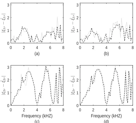
To immediately illustrate the need for improvement in EM estimates of the frequency domain GMM arising in the source separation algorithms described above, a comparison of the EM estimates of the ILD mean parameter µˆ(ω) computed using the algorithm of [8] with the ground-truth values µ(ω)
is provided in Fig. 2. It displays the ground-truth ILD mean (black) and its EM estimate (grey) for two-source binaural mixtures formed by convolving two randomly chosen speech signals from the TIMIT data set with impulse responses measured by Hummersone [28] under anechoic (Room A) and reverberant conditions (Room DwithRT60= 0.89s), with the
two sources placed at0◦ and30◦(further details are provided in section VI). The top row of the plot corresponds to (a) µ1(ω) – the ILD mean for s1, and (b) µ2(ω) – the ILD
mean for s2, for the anechoic mixture; subplots (c) and (d)
similarly correspond to the ILD mean for s1 and s2 in the
reverberant room. Clearly, the estimated ILD mean follows the ground truth ILD very closely for the anechoic case, especially for source 2 (Fig. 2(b)). On the other hand, we see large variation in the EM estimates of the ILD mean parameter, [8] in the reverberant case. In this section, we describe the bootstrap averaging algorithm to yield improved estimates of the frequency domain GMM parameters (in Γ) employed in the framework of [8].
A convenient way to bootstrap the frequency-dependent GMM parameter estimates is to bootstrap the observed mixture vector
x=[x(1) . . . x(N)]= [
l(1) . . . l(N)
r(1) . . . r(N) ]
to obtain time domain bootstrap samples, denoted as
x∗1, . . . ,x∗B from which bootstrap estimates of the cue model parameters can be obtained directly using the algorithm of [8]. Since model-based source separation relies on the interaural spectrogram derived from the speech mixture vector, it is important to use a bootstrap procedure that appropriately mimics the frequency domain dependence in the given sample. Bootstrap samples of the mixture vector are obtained using the circulant embedding based approach of [25]. The basic idea in [25] is to generate portions of realizations with spectral density given by an estimated spectral density derived from the ob-served vector-valued time series via circulant embedding. The procedure of [25] is easily implemented using a FFT which
0 2 4 6 8
−5 0 5
ILD (dB)
(a)
0 2 4 6 8
−20 −10 0 10
(b)
0 2 4 6 8
−5 0 5
Frequency (kHz) (c)
ILD (dB)
0 2 4 6 8
−20 −10 0 10
[image:8.612.329.537.66.251.2]Frequency (kHz) (d)
Fig. 2. The mean ILD estimatesµi(ω)ˆ (solid grey) from the joint model of [8] vs. frequency (kHz) in an anechoic environment for (a)i = 1and (b)
i= 2; and a reverberant (Room D,RT60= 0.89s – see sec. VI for further
details) room environment for (c)i= 1and (d)i= 2. The solid black line in each subplot shows the ground-truth ILD mean (dB)µi(ω). Sourcess1and s2 chosen from the TIMIT data set were placed atφ= 0◦, andφ= 30◦,
respectively.
makes it computationally efficient and hence very attractive for our application where the length-N of the observed speech mixtures is usually very large.
Consider a bivariate discrete time second-order stationary process Vt = [Xt, Yt]T, where t ∈ Z denotes the time
index. Without loss of generality, assume that each component process has a mean of zero. Given a length-N realization
V1, . . . ,VN from the vector process Vt, the following
boot-strap algorithm [25], allows us to generate bootboot-strap time series samples.
Bootstrap algorithm:
1) Choose the embedding size m1 > 2(N−1) such that
m1 = 2g for some g ∈ Z+. Estimate the spectral
matrix SˆV(fl), fl = l/(m1∆) , l = 0,1, . . . , m1−1,
with ∆ denoting the sampling interval, using one of the recommended spectral estimation methods [25], such as multitaper, Welch’s Overlapped Segment Averaging (WOSA) etc.
2) Set λl = ˆST
V(fl)/∆, l = 0, . . . , m1−1. For each l = 0, . . . , m1−1, determine the2×2unitary matrixUland
the diagonal matrixDl such thatλl=UlDlUHl , where
.H denotes conjugate transpose.
3) Simulate two real bivariate independent standard normal vectors Zl(α) ∼ N(0,I2);α = 1,2, and set Cl =
UlD 1/2 l (Z
(1)
l + iZ
(2) l ).
4) Define V˜j = m− 1/2 1
∑m1−1
l=0 Cle−
i2πlj/m1, j =
0, . . . , m1 −1, which can be computed easily via an
FFT. Then for eachj, V˜j is a complex-valued bivariate
vector. Re{V˜n}, n= 0,1, . . . , N −1 and Im{V˜n}, n= 0,1, . . . , N −1 are two independent length-N bootstrap replications.
bootstrap samples have the specified second-order structure. This has also been verified empirically, [24].
Note that most of the existing bootstrap procedures are only applicable to second-order stationary data. Since short segments of speech (30−50ms) are considered to be second-order stationary [30], we shall apply the bootstrap procedure to short segments of the observed speech mixture. The algorithm for bootstrap-based source separation under the model-based framework of [8] is outlined below.
(i) Divide x ≡ [x(1), . . . ,x(N)] into adjacent pseudo second-order stationary blocks of length-N˜. The jth block is given by
zj=x(2−j+ (j−1) ˜N: 1 +j( ˜N−1));
j= 1, . . . , Nb, whereNb denotes the number of blocks
required to cover the full length-N ofx. For eachj,zj
is a matrix of size2×N.˜
(ii) For each block zj, implement the bootstrap algorithm
of [25] (given above), to generateB bootstrap samples, each of lengthN˜−1(to avoid generating the end point twice due to adjacent blocks). So for the jth block, j= 1, . . . , Nb,obtainz∗j,b, b= 1, . . . , B. For each block,
the algorithm of [25] is implemented with the multitaper spectral estimation technique, which for a given
length-˜
N bivariate time serieszis a2×2 matrix given by:
ˆ
Sz(ω) =
∆
P
P ∑
p=1
˜ N ∑
n=1
un,pz(n)e−i2πωn∆
2
, (22)
where |ω| ≤ 1/(2∆), and {un,p} ˜ N
n=1 is the pth data
taper. Tapering prevents the spectra from the problem of leakage and the application ofP orthogonal data tapers as in the multitaper approach leads to a consistent spec-tral estimate [31]. Then the bth full length-N bootstrap sample forxis given by
x∗b =[z∗1,b . . . z∗N
b,b
]
2×N,
andx∗1, . . . ,x∗B are theB bootstrap samples.
(iii) The source separation algorithm of [8] is applied to each of the B bootstrap samples x∗1, . . . ,x∗B, in-dividually. This leads to B bootstrap estimates for each parameter in Γiτ. For each i and τ, let Γ∗iτ,1, . . . ,Γ∗iτ,B denote the bootstrap parameter set where Γ∗iτ,b = {a∗i,b(ω), σ∗i,b(ω), ξiτ,b∗ (ω), γiτ,b∗ (ω), µ∗i,b(ω), ηi,b∗ (ω), ψ∗iτ,b} contains model parameter esti-mates derived from the bth bootstrap sample x∗b. This is used to construct the bootstrap averaged estimates for each frequency dependent parameter.
(iv) The algorithm of [8] allows us to compute bootstrap T-F masks M∗i,b = [Mi,b∗ (ω, t)] ∈ [0,1]W×T corresponding to the bootstrap estimates of GMM parameters in Γ∗iτ,b
using each of the b = 1, . . . , B bootstrap replications. The averaged bootstrap T-F mask given by M∗i,A = [Mi,∗A(ω, t)]where
Mi,∗A(ω, t) = M
∗
i,1(ω, t) +. . .+Mi,B∗ (ω, t)
B , (23)
is used for recovering the source vectorss1, . . . ,sI from
the observed speech mixture vectors inx.
Note that the time-frequency mask given by (20) is a by-product of the EM algorithm, computed using the output of the E-step (19) which gives the probability of a spectrogram point (ω, t) coming from source i and delay τ, conditional on the interaural cues α(ω, t) and ϕ(ω, t) (estimated using the spectrogram of the observed speech mixture), in addition to the parameter estimates from the final M-step of the EM algorithm. For each bootstrap replication, the E-step allows us to compute this probability or T-F masks, conditional on the interaural cuesα∗(ω, t)andϕ∗(ω, t), estimated from the spec-trogram of the bootstrap speech mixture. From [24, Chapter 7], we know that the bootstrap procedure leads to samples which replicate the true frequency domain statistics, i.e. the spectra of bootstrap samples, on average, mimics the theoretical spectra of the process generating the observed sample. Thus, if the bootstrap averaged GMM parameter estimates lead to a smaller MSE in comparison with the original EM estimates, each bootstrap F mask is a reasonable estimate (of the true T-F mask). The average of the bootstrap T-T-F masks provides a simple way to construct an overall T-F mask based on the bootstrap data. We verify the performance of the bootstrap averaged estimates and the bootstrap averaged T-F mask for the task of source separation in our experiments below.
VI. EXPERIMENTS ANDRESULTS
A. Set-up
We present the experimental set-up used to test the pro-posed bootstrap averaging technique for source separation as described above using speech mixtures formed with real room-recorded impulse responses. We use the TIMIT data set from which15utterances are randomly selected to form convolutive mixtures using binaural room impulse responses (BRIRs), [8]. The BRIRs were captured by Hummersone [28] using a Head and Torso Simulator (HATS). The HATS and the sources were placed at a height of2.8m in the room and were separated by a distance of1.5m. The target source is placed exactly in front of HATS, i.e. at zero degree relative to HATS and the two interfering sources are positioned symmetrically on the left and right hand side of the target source in an arc at azimuth denoted by φ (in degrees). The BRIRs were measured in 5
different rooms corresponding to five different reverberation levels given byRT60 and azimuths ranging from−90◦ to90◦
at 5◦ intervals. The sampling frequency denoted as fs is 16
kHz and the sampling interval is ∆ = 1s. From the chosen set of 15utterances, we combined two (three) speech signals (about3s, shortened to2.5s for consistency) with BRIRs from Room Dwhich corresponds to the highest reverberation time of 0.89s within the recorded data set to construct two sets of mixtures: (i)15two-source mixtures, and (ii)15three-source mixtures, for each azimuthφ= 15◦,30◦,45◦,60◦,75◦.
To implement the algorithm described in section V, we dividex into pseudo stationary blocks of length30ms which correspond toN˜ =fs×0.003 = 16000×0.003 = 480samples
the bivariate time series in each block are computed as given in (22). We employ P = 8sine tapers{un,p}, where
un,p= 2
( ˜N+ 1)1/2sin
(p+ 1)πn
˜
N+ 1 , n= 1, . . . , ˜
N , (24)
leading to a bandwidth of WN˜ = (P + 1)/2( ˜N + 1) = 0.0094 [31]. Then following the steps in section V, the simulation procedure of [25] is applied to the time series in each block with B = 500 to obtain B bootstrap samples
x∗1, . . . ,x∗Bof the full length-N speech mixture. Next, param-eter sets Γ∗iτ,1, . . . ,Γ∗iτ,B containing bootstrap estimates and time-frequency masks M∗i,1, . . . ,M∗i,B for each source index i = 1, . . . , I, and admissible τ are derived using the source separation algorithm of [8]. We conduct all our experiments with the additionalgarbage sourcewhich aims to account for spectrogram points where reverberation (rather than one of the I sources) dominates, [1].
B. Comparison of Cue Parameter Estimates
Here we focus on estimates of the frequency domain GMM parameters, i.e. elements ofΓ. We compare estimates obtained using the algorithm of [8], and the bootstrap averaged esti-mates, with their ground-truth values. Here ground-truth refers to the parameter values that would be obtained if each source was observed in isolation. We focus on the ILD, IPD, and the mixing vector cue mean parameters. The ground-truth for these parameters is obtained as described below. The ground-truth ILD mean is computed from the isolated one-source direct-path mixture, i.e. µi is obtained by convolving only
the ith source with the direct-path impulse response denoted as [˜hil(n),˜hir(n)]T to form the convolutive mixture vector
˜
x(i)(n) = [˜li(n),r˜i(n)]T, where ˜. denotes direct-path and superscript .(i) indicates that the mixture only involves the
ith source. Then from the definition of ILD, it follows that
µi(ω) = 1
T
T ∑
t=1
20 log10 | ˜
L(i)(ω, t)|
|R˜(i)(ω, t)|, (25)
where [ ˜L(i)(ω, t)]
W×T, and [ ˜R(i)(ω, t)]W×T denote the
STFTs of direct path mixture vectors [˜li(1), . . . ,˜li(N)] and [˜ri(1), . . . ,r˜i(N)], respectively. Alternatively, from [1], the
ground-truth ILD mean may be computed directly from the direct-path impulse response as
µi(ω) = 20 log10
(
|H˜il(ω)| |H˜ir(ω)|
)
, (26)
where H˜il = F{h˜il}, and similarly, H˜ir = F{˜hir}, F{.}
denoting the Fourier transform.
Similarly, the ground-truth IPD residual mean for the ith source is given by, [1]:
ξiτ(ω) = arg (
e−i ˜ϕ(ω,t)e−iωτ(ω) )
, (27)
where ϕ˜(ω, t) =arg( ˜Hil(ω)/H˜ir(ω)), and τ(ω) =τl−τr+
arg( ¯Hil(ω)/H¯ir(ω)), with H¯il(ω) = F{¯hil(n)}, H¯ir(ω) = F{¯hir(n)} andh¯il(n),¯hir(n)denoting the impulse response
truncated at the length of the analysis window. Also arg(.)
denotes the argument, taking values in the interval(−π, π].
Since ai(ω) denotes the mean of the reverberant mixture
vector in the T-F domain, the ground-truth mixing vector meanai(ω)is computed as described in [9] from the isolated
mixture ˇx(i)(n) = [ˇli(n),rˇi(n)]T, whereˇ. indicates that the
ith source is convolved with the full impulse response. The corresponding EM estimates and bootstrap averaged estimates for each GMM parameter are computed using the algorithm of [8] and bootstrap as described above in section V and VI-A.
Due to the non-identifiability of GMMs, it is important to learn the permutation that allows consistent averaging across bootstrap estimates for each parameter. We described in section III-A, how this may be achieved using the fact that the component variances are well-separated. Different ways to solve the permutation problem due to EM estimation have been studied in the blind source separation literature. In the case of a frequency specific GMM, as in the algorithms of [9], [1], and [8], dealing with the permutation problem is crucial to be able to group together components corresponding to the same source estimated at each frequency. Traditionally, correlation coefficients ofamplitude envelopeswhich represent sound source activity, are used to identify the permutation, for example, [32], [33], however, more recently efficient approaches as in [9], have been discussed and are commonly employed. Other techniques solving the permutation problem for frequency domain source separation are discussed in [34] and [35]. Thus, applications employing the EM algorithm for frequency domain source separation commonly have a built-in strategy to deal with the permutation problem, allowing us to average the component parameter estimates consistently across bootstrap replications.
Consider the set of two-source mixtures with the target sources1atφ= 0◦and the interference sources2atφ= 30◦.
For convenience, we label the 15 two-source mixtures as k′ = 1, . . . ,15. Fig. 3 shows a comparison of the ILD mean estimates µˆi(ω) obtained from the model-based method of
[8] (solid grey), and the bootstrap-based estimates µˆi,A(ω) (solid black), with the ground-truth estimates µi(ω) (dashed
black) over the frequency range (kHz) [0, fs/2∆] = [0,8].
The dotted black lines show the ground-truth ILD mean of each source convolved with impulse response truncated to the length of our analysis window. Note that it follows the direct path ILD mean (dashed black) very closely but has a relatively higher variation. This is due to the early echoes in the impulse response truncated at the window length. The subplots in the left column of Fig. 3 correspond toµ1(ω), i.e.
the ILD mean parameter for the target source with subplots in consecutive rows corresponding to the first four mixtures, i.e. k′ = 1,2,3,4, respectively; similarly, the subplots in the right column correspond to µ2(ω), the ILD mean parameter
for the interference source for k′ = 1,2,3,4, respectively. From the figure we see that the bootstrap averaged ILD mean estimatesµˆ∗i,A(ω)(solid black) follow the ground-truthµi(ω)
(dashed black) very closely; ILD mean estimatesµˆi(ω)(solid
grey) obtained from the joint method of [8] evidently show large deviations from the ground-truth at each frequency. For a clearer comparison, we compare the absolute error inµˆi(ω)
0 2 4 6 8 (a) -5 0 5 ILD (dB)
0 2 4 6 8
(b) -20
-10 0 10
0 2 4 6 8
(c) -5
0 5
ILD (dB)
0 2 4 6 8
(d) -20
-10 0 10
0 2 4 6 8
(e) -5
0 5
ILD (dB)
0 2 4 6 8
(f) -20
-10 0 10
0 2 4 6 8
Frequency (kHz) (g) -5 0 5 ILD (dB)
0 2 4 6 8
Frequency (kHz) (h) -20 -10 0 10
Fig. 3. A comparison of the ground-truth ILD mean (dB) µi(ω)(dashed black) with the estimate µi(ω)ˆ (solid grey) obtained from [8], and the bootstrap averaged estimate µˆ∗i,A(ω) (solid black) vs. frequency (kHz) for (a)i= 1, k′ = 1, (b)i= 2, k′= 1, (c)i= 1, k′= 2, (d)i= 2, k′= 2, (e)i= 1, k′= 3, (f)i= 2, k′= 3, (g)i= 1, k′= 4, and (h)i= 2, k′= 4
withs1 placed atφ= 0◦, ands2placed atφ= 30◦. The ground-truth ILD
mean of each source convolved with impulse response truncated to the window length are shown in dotted black.
0 2 4 6 8
(a) 0 1 2 3 4 5 | µ1 − ˆ µ1 |
0 2 4 6 8
(b) 0 1 2 3 4 5 | µ1 − ˆ µ1 |
0 2 4 6 8
Frequency (kHZ) (c) 0 5 10 15 | µ2 − ˆ µ2 |
0 2 4 6 8
[image:11.612.328.552.68.270.2]Frequency (kHZ) (d) 0 5 10 15 | µ2 − ˆ µ2 |
Fig. 4. A comparison of the absolute errors in the ILD mean (dB) estimate
ˆ
µi(ω)from [8] (solid grey), and the bootstrap averaged estimate µˆ∗i,A(ω)
(dashed black) vs. frequency (kHz), for (a)i= 1, k′= 1, (b)i= 1, k′= 2, (c)i= 2, k′= 1, and (d)i= 2, k′= 2. The asterisk∗denotes the frequency of interest in each case.
(solid grey) andµˆ∗i,A(ω)(dashed black) for source and mixture combinations corresponding to the two sources and the first two mixtures, i.e. (a) i = 1, k′ = 1, (b) i = 1, k′ = 2, (c) i= 2,k′= 1and (d)i= 2,k′ = 2. For clarity, we have only plotted absolute errors for a set of equally spaced frequencies. From Fig. 4(a)-(b) it is clear thatµˆ∗1,A(ω)outperformsµˆ1(ω)
at all frequencies, however, fori= 2, we observe frequencies whereµˆ2(ω)has a smaller error as compared toµˆ∗2,A(ω). The
0 2 4 6 8
(a) 0
1 2 3
0 2 4 6 8
(b) 0
1 2 3
0 2 4 6 8
Frequency (kHZ) (c) 0 1 2 3
0 2 4 6 8
[image:11.612.68.293.70.264.2]Frequency (kHZ) (d) 0 1 2 3
Fig. 5. A comparison of the absolute errors in the IPD mean estimateξiτˆ (ω)
from [8] (solid grey), and the bootstrap averaged estimateξˆ∗A,iτ(ω)(dashed black) vs. frequency (kHz) for (a)i = 1, k′ = 1, (b)i = 1, k′ = 3, (c)
i= 2, k′= 1,, (d)i= 2, k′= 3at the ground truth delayτ= 4.
frequencies marked with∗depict four different scenarios and are discussed in the next subsection. Similarly, Fig. 5 displays
0 2 4 6 8
(a) 0 0.5 1 1.5 | a1 l − ˆ a1 l |
0 2 4 6 8
(b) 0 0.5 1 1.5 | a1 l − ˆ a1 l |
0 2 4 6 8
Frequency (kHZ) (c) 0 0.5 1 1.5 2 | a1 r − ˆ a1 r |
0 2 4 6 8
Frequency (kHZ) (d) 0 0.5 1 1.5 | a1 r − ˆ a1 r |
Fig. 6. A comparison of the absolute error in the mixing vector mean estimate
ˆ
a1(ω)(solid grey) from [8], and the bootstrap averaged estimateaˆ∗1,A(ω)
(dashed black) vs. frequency (kHz) for the left componental1(ω)of mixtures
(a)k′= 2, (b)k′= 4, and for the right componentar1(ω)of mixtures (c) k′= 2, and (d)k′= 4.
absolute error in the IPD mean estimatesξˆiτ(ω) (solid grey)
[image:11.612.63.287.380.575.2] [image:11.612.323.549.383.565.2]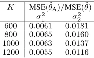
![Fig. 2. The mean ILD estimates ˆ[8] vs. frequency (kHz) in an anechoic environment for (a)details) room environment for (c)sµi(ω) (solid grey) from the joint model of i = 1 and (b)i = 2; and a reverberant (Room D, RT60 = 0.89s – see sec](https://thumb-us.123doks.com/thumbv2/123dok_us/8851452.935056/8.612.329.537.66.251/estimates-frequency-anechoic-environment-details-environment-solid-reverberant.webp)
![Fig. 8. A comparison of the average SDR over a set of (a) 15mixtures, and (b)the proposed technique (square), the integrated method of [8] (asterisk), theinteraural cue-based technique of [1] (circle), and the mixing vector modelbased method of [9] (dot) f](https://thumb-us.123doks.com/thumbv2/123dok_us/8851452.935056/13.612.75.276.65.237/comparison-mixtures-proposed-technique-integrated-theinteraural-technique-modelbased.webp)
