Saliency propagation from simple to difficult

BIROn - Birkbeck Institutional Research Online

Gong, C. and Tao, D. and Wei, L. and Maybank, Stephen and Meng,

F. and Fu, K. and Yang, Jie (2015) Saliency propagation from simple to

difficult.

IEEE Computer Society Conference on Computer Vision and

Pattern Recognition , pp. 2531-2539. ISSN 1063-6919.

Downloaded from:

Usage Guidelines:

Please refer to usage guidelines at

or alternatively

Saliency Propagation from Simple to Difficult

Chen Gong

, Dacheng Tao

, Wei Liu

, S.J. Maybank

, Meng Fang

, Keren Fu

, and Jie Yang

1

_{Institute of Image Processing and Pattern Recognition, Shanghai Jiao Tong University}

_{The Centre for Quantum Computation & Intelligent Systems, University of Technology, Sydney}

3

_{IBM T. J. Watson Research Center}

_{Birkbeck College, London}

Please contact: [email protected]; [email protected]

June 9, 2016

Abstract

Saliency propagation has been widely adopted for identifying the most attractive object in an image. The prop-agation sequence generated by existing saliency detection methods is governed by the spatial relationships of image regions,i.e., the saliency value is transmitted between two adjacent regions. However, for the inhomogeneous dif-ficult adjacent regions, such a sequence may incur wrong propagations. In this paper, we attempt to manipulate the propagation sequence for optimizing the propagation quality. Intuitively, we postpone the propagations to difficult regions and meanwhile advance the propagations to less ambiguous simple regions. Inspired by the theoretical results in educational psychology, a novel propagation algorithm employing the teaching-to-learn and learning-to-teach s-trategies is proposed to explicitly improve the propagation quality. In the teaching-to-learn step, a teacher is designed to arrange the regions from simple to difficult and then assign the simplest regions to the learner. In the learning-to-teach step, the learner delivers its learning confidence to the learning-to-teacher to assist the learning-to-teacher to choose the subsequent simple regions. Due to the interactions between the teacher and learner, the uncertainty of original difficult regions is gradually reduced, yielding manifest salient objects with optimized background suppression. Extensive experi-mental results on benchmark saliency datasets demonstrate the superiority of the proposed algorithm over twelve representative saliency detectors.

1

Introduction

Saliency detection has attracted intensive attention and achieved considerable progress during the past two decades. Up to now, a great number of detectors based on computational intelligence have been proposed. They can be roughly divided into two categories:bottom-upmethods that are data and stimulus driven, andtop-downmethods that are task and knowledge driven.

Top-down methods are usually related to the subsequent applications. For example, Maybank [21] proposed a probabilistic definition of salient image regions for image matching. Yanget al. [28] combined dictionary learning and Conditional Random Fields (CRFs) to generate discriminative representation of target-specific objects.

Different from top-down methods, bottom-up methods use low-level cues, such as contrast and spectral informa-tion, to recognize the most salient regions without realizing content or specific prior knowledge about the targets. The representatives include [11,10,16,4,22,19,14,17,8].

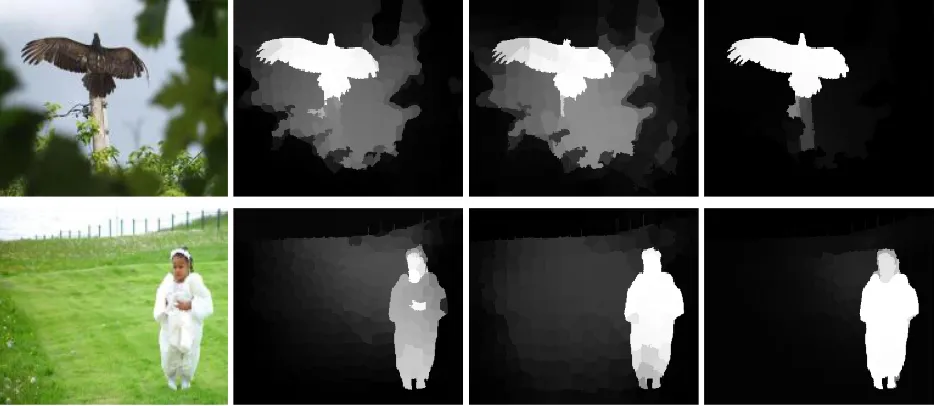
Figure 1: The results achieved by typical propagation methods and our method on two example images. From left to right: input images, results of [27], [12], and our method.

inhomogeneous or incoherent adjacent superpixels, the propagation sequences are misleading and likely to lead to inaccurate detection results (see Fig.1).

Based on the above observations, we argue that not all neighbors are suitable to participate in the propagation process, especially when they are inhomogeneous or visually different from the labeled superpixels. Therefore, we assume different superpixels have different difficulties, and measure the saliency values of the simple superpixels prior to the difficult ones. This modification to the traditional scheme of generating propagation sequences is very critical, because in this modification the previously attained knowledge can ease the learning burden associated with complex superpixels afterwards, so that the difficult regions can be precisely discovered. Such a “starting simple” strategy conforms to the widely acknowledged theoretical results in pedagogic and cognitive areas [5,23,13], which emphasize the importance of teachers for human’s acquisitions of knowledge from the childish stage to the mature stage.

By taking advantage of these psychological opinions, we propose a novel approach for saliency propagation by leveraging a teaching-to-learn and learning-to-teach paradigm (displayed in Fig.3). This paradigm plays two key roles: a teacher behaving as a superpixel selection procedure, and a learner working as a saliency propagation procedure. In the teaching-to-learn step of thet-th propagation, the teacher assigns the simplest superpixels (i.e., curriculum) to the learner in order to avoid the erroneous propagations to the difficult regions. Theinformativity,individuality,

inhomogeneity, andconnectivityof the candidate superpixels are comprehensively evaluated by the teacher to decide the proper curriculum. In the learning-to-teach step, the learner reports itst-th performance to the teacher in order to assist the teacher in wisely deciding the(t+ 1)-th curriculum. If the performance is satisfactory, the teacher will choose more superpixels into the curriculum for the following learning process. Owing to the interactions between the teacher and learner, the superpixels are logically propagated from simple to difficult with the updated curriculum, resulting in more confident and accurate saliency maps than those of typical methods (see Fig.1).

2

Saliency Detection Algorithm

input image convex hull _{(blue polygon)} & superpixels

graph construction (white lines are

edges)

background seeds

boundary seeds

convex hull mask

coarse saliency

map final saliency map

superpixels

Pre-processing

Stage 2

Stage 1

②

①

③

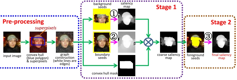
Figure 2: The diagram of our detection algorithm. The magenta arrows annotated with numbers denote the implemen-tations of teaching-to-learn and learning-to-teach propagation shown in Fig.3.

2.1

Image Pre-processing

Given an input image, a convex hullHis constructed to estimate the target’s location [26]. This is done by detecting some key points in the image via Harris corner detector. Because most key points locate within the target region, we link the outer key points to a convex hull to roughly enclose the target (see Fig.2).

We proceed by using the SLIC [1] algorithm to over-segment the input image intoN small superpixels (see Fig.

2), then an undirected graphG=hV,Eiis built whereVis the node set consisted of these superpixels andEis the edge set encoding the similarity between them. In our work, we link two nodes1_s

iandsjby an edge if they are spatially

adjacent in the image or both of them correspond to the boundary superpixels. Then their similarity is computed by

the Gaussian kernel functionωij = exp

−ksi−sjk

2

/(2θ2_{), whereθis the kernel width ands}

iis the feature vector

of thei-th superpixel represented in the LAB-XY space (i.e. si = (scolori ;s position

i )). Therefore, theG’s associated

adjacency matrixW∈RN×N is defined byWij =ωijifi6=j, andWij= 0otherwise. The diagonal degree matrix

isDwithDii=PjWij.

2.2

Coarse Map Establishment

A coarse saliency map is built from the perspective of background, to assess how these superpixels are distinct from the background. To this end, some regions that are probably background should be determined as seeds for the saliency propagation. Two background priors are adopted to initialize the background propagations. The first one is theconvex hullprior [26] that assumes the pixels outside the convex hull are very likely to be the background; and the second one is theboundary prior[24,27] which indicates the regions along the image’s four boundaries are usually non-salient.

For employing the convex hull prior, the superpixels outsideHare regarded as background seeds (marked with yellow in Fig. 2) for saliency propagation. Suppose the propagation result is expressed by anN-dimensional vector

f∗ = f₁∗ · · · f_N∗T

, wheref_i∗(i = 1,· · ·, N) are obtained saliency values corresponding to the superpixelssi,

then after scalingf∗to[0,1](denoted asf_normalized∗ ), the value of thei-th superpixel in the saliency mapSConvexHull

is

SConvexHull(i) = 1−fnormalized∗ (i), i= 1,2,· · ·, N, (2.1)

Similarly, we treat the superpixels of four boundaries as seeds, and implement the propagation again. A saliency map based on the boundary prior can then be generated, which is denoted asSBoundary. Furthermore, we establish a

binary maskSmask[7] to indicate whether thei-th superpixel is inside (SM ask(i) = 1) or outside (SM ask(i) = 0) the

convex hullH. Finally, the saliency map of Stage 1 is obtained by integratingSConvexHull,SBoundary, andSM askas

SStage1=SConvexHull⊗SBoundary⊗SM ask, (2.2)

where “⊗” is the element-wise product between matrices.

2.3

Map Refinement

After the Stage 1, the dominant object can be roughly highlighted. However,SStage1may still contain some back-ground noise that should be suppressed. Therefore, we need to propagate the saliency information from the potential foreground regions to further improveSStage1.

Intuitively, we may choose the superpixels with large saliency values inSStage1as foreground seeds. In order to avoid erroneously taking background as seeds, we carefully pick up a small number of superpixels as seeds that are in the set:

{si|SStage1(i)≥ηmax1≤j≤N(SStage1(j))}, (2.3) whereηis set to 0.7. Finally, by setting the labels of seeds to 1 and conducting the teaching-to-learn and learning-to-teach propagation, we achieve the final saliency mapSStage2. Fig. 2illustrates thatSStage2successfully highlights the foreground regions while removes the background noise appeared inSStage1.

3

Teaching-to-learn and Learning-to-teach For Saliency Propagation

Saliency propagation plays an important role in our algorithm. Suppose we havel seed nodess1,· · ·,sl onGwith

saliency valuesf1=· · ·=fl= 1, the task of saliency propagation is to reliably and accurately transmit these values

from thellabeled nodes to the remainingu=N−lunlabeled superpixels.

As mentioned in the introduction, the propagation sequence in existing methods [9,27,12] may incur imperfect results on difficult superpixels, so we propose a novel teaching-to-learn and learning-to-teach framework to optimize the learning sequence (see Fig.3). To be specific, this framework consists of a learner and a teacher. Given the labeled set and unlabeled set at timetdenoted asL(t)_andU(t)_{, the teacher selects a set of simple superpixels fromU}(t)_as curriculumT(t)_{. Then, the learner will learnT}(t)_{, and return a feedback to the teacher to help the teacher update the} curriculum for the(t+ 1)-th learning. This process iterates until all the superpixels inU(t)_{are properly learned.}

3.1

Teaching-to-learn

The core of teaching-to-learn is to design a teacher deciding which unlabeled superpixels are to be learned. For the t-th propagation, a candidate setC(t)_{is firstly established, in which the elements are nodes directly connected to the} labeled setL(t)_{onG. Then the teacher chooses the simplest superpixels fromC}(t)_{as thet-th curriculum. To evaluate} the propagation difficulty of an unlabeled superpixel si ∈ C(t), the difficulty scoreDSi is defined by combining

informativityIN Fi, individualityIN Di, inhomogeneityIHMi, and connectivityCONi, namely:

DSi=IN Fi+β1IN Di+β2IHMi+β3CONi, (3.1)

whereβ1,β2andβ3are weighting parameters. Next we will detail the definitions and computations ofIN Fi,IN Di,

IHMi, andCONi, respectively.

Informativity:The simple superpixel should not contain too much information given the labeled setL2_{. Therefore,}

the informativity of a superpixelsi∈ Cis straightforwardly modelled by the conditional entropyH(si|L), namely:

IN Fi=H(si|L). (3.2)

The propagations on the graph follow the multivariate Gaussian process [31], with the elementsfi(i= 1,· · · , N)

in the random vectorf = f1 · · · fN T

denoting the saliency values of superpixelssi. The associated covariance

matrixKequals to the adjacency matrixWexcept the diagonal elements are set to 1. For the multivariate Gaussian, the closed-form solution ofH(si|L)is [3]:

H(si|L) =

1

2ln(2πeσ 2

i|L), (3.3)

whereσ2

i|Ldenotes the conditional covariance offigivenL. Considering that the conditional distribution is a

multi-variate Gaussian,σ2

i|Lin (3.3) can be represented by

σ2_i|L=K2_ii−Ki,LK−L,1LKL,i, (3.4)

in whichKi,L andKL,L denote the sub-matrices ofKindexed by the corresponding subscripts. By plugging (3.3)

and (3.4) into (3.2), we obtain the informativity ofsi.

informativity

individuality

connectivity

integrated

updated

labeled

superpixels

Teaching-to-learn

Learning-to-teach

labeled

superpixels

Learning confidence

saliency map

iterate

inhomogeneity

In (3.4), the inverse of anl×l(lis the size of gradually expanded labeled setL) matrixKL,Lshould be computed

in every iteration. Aslbecomes larger and larger, directly inverting this matrix can be time-consuming. Therefore, an efficient updating technique is developed in thesupplementary materialbased on the blockwise inversion equation. Individuality: Individuality measures how distinct of a superpixel to its surrounding superpixels. We consider a superpixel simple if it is similar to the nearby superpixels in the LAB color space. This is because such superpixel is very likely to share the similar saliency value with its neighbors, thus can be easily identified as either foreground or background. For example, the superpixels2in Fig.4(a) has lower individuality thans1since it is more similar to the neighbors thans1. The equation below quantifies the local individuality ofsiand its neighboring superpixelsN(si):

IN Di=IN D(si,N(si)) =

1

|N(si)|

X

j∈N(si)

s

color i −s

color j

, (3.5)

where|N(si)| denotes the amount of si’s neighbors. Consequently, the superpixels with small individuality are

preferred for the current learning.

Inhomogeneity:It is obvious that a superpixel is ambiguous if it is not homogenous or compact. Fig.4(b) provides an example that the homogenouss4gets smallerIHMthan the complicateds3. Suppose there arebpixels

pcolor j

b j=1 in a superpixelsi characterized by the LAB color feature, then their pairwise correlations are recorded in the b×

b symmetric matrix Θ = PPT, where Pis a matrix with each row representing a pixelpcolor_j . Therefore, the inhomogeneity of a superpixelsiis defined by the reciprocal of mean value of all the pairwise correlations:

IHMi=

2 b2_−b

Xb

i=1

Xb

j=i+1Θij

−1

, (3.6)

whereΘijis the(i, j)-th element of matrixΘ. SmallIHMimeans that all the pixels insiare much correlated with

others, sosiis homogenous and can be easily learned.

Connectivity:For the established graphG, a simple intuition is that the nodes strongly connected to the labeled setL

are not difficult to propagate. Such strength of connectivity is inversely proportional to the averaged geodesic distances betweensi∈ Cand all the elements inL, namely:

CONi =

1 l

X

j∈Lgeo(si,sj). (3.7)

In (3.7),geo(si,sj)represents the geodesic distance betweensiandsj, which can be approximated by their shortest

path, namely:

geo(si,sj) = min R1=i,R2,···,Rn=j

Xn−1

k=1max(ERk,Rk+1−c0,0) s.t. Rk, Rk+1∈ V, RkandRk+1are connected inG

. (3.8)

HereV denotes the nodes set ofG,ERk,Rk+1 computes the Euclidean distance betweenRk andRk+1, andc0is an

adaptive threshold preventing the “small-weight-accumulation” problem [24].

Finally, by substituting (3.2), (3.5), (3.6) and (3.7) into (3.1), the difficulty scores of allsi∈ Ccan be calculated,

based on which the teacher is able to determine the simple curriculum for the current iteration. With the teacher’s effort, the unlabeled superpixels are gradually learned from simple to difficult, which is different from the propagation sequence in many existing methodologies [27,12,9]. Suppose there are|C|superpixels in candidate setC, then the weighting parametersβ1,β2andβ3in (3.1) are decided by



 

 

β1= var IN D1,· · · , IN D|C|

/var IN F1,· · ·, IN F|C|

β2= var IHM1,· · · , IHM|C|

/var IN F1,· · · , IN F|C|

β3= var CON1,· · · , CON|C|

/var IN F1,· · ·, IN F|C|

, (3.9)

wherevar(·)is the variance computation operator. In (3.9), the metric with large variance is assigned to large weight, because it properly reflects the difference of candidate superpixels.

3.2

Learning-to-teach

After the difficulty scores of all candidate superpixels are computed, the next step is to pick up a certain number of superpixels as curriculum based onDS1,· · ·, DS|C|. A straightforward idea is to sort all the elements inCso that their

difficulty scores satisfyingDS1≤DS2≤ · · · ≤DS|C|. Then the firstq(q≤ |C|) superpixels are used to establish the

(a)

(b)

Figure 4: The illustrations of individuality (a) and inhomogeneity (b). The regions1in (a) obtains larger individuality thans2, ands3in (b) is more inhomogeneous thans4.

be learned attshould depend on the(t−1)-th learning performance. If the(t−1)-th learning is confident, the teacher may assign “heavier” curriculum to the learner. In other words, the teacher should also consider the learner’s feedback to arrange the proper curriculum, which is a “learning-to-teach” mechanism. Next we will use this mechanism to adaptively decideq(t)_{for thet-th curriculum.}

As mentioned above,q(t) _{should be adjusted by considering the effect of previous learning. However, since the} correctness of the(t−1)-th output saliency is unknown, we define a confidence score to blindly evaluate the previous learning performance. Intuitively, the(t−1)-th learning is confident if the saliency valuesf₁(t−1),· · · , f_q((t−t−1)1)are close

to 0 (very dissimilar to seeds) or 1 (very similar to seeds) after scaling. However, iff₁(t−1),· · · , f_q(t(−t−1)1) are close to the

ambiguous value 0.5, the teacher will rate the last learning as unsatisfactory, and produce a smallq(t)_{to relieve the} “burden” for the current learning. Therefore, the confidence score that belongs to[0,1]is defined by

Conf idenceScore=1− 2

q(t−1)

Xq(t

−1)

i=1min(f (t−1)

i ,1−f

(t−1)

i ), (3.10)

andq(t)is finally computed by

q(t)=Ct

×Conf idenceScore

. (3.11)

3.3

Saliency Propagation

After the curriculumT(t)₌

s1,s2,· · ·,sq(t) is specified, the learner will spread the saliency values fromL(t)to

T(t)_{via propagation. Particularly, the expression is:}

f(t+1)=M(t)D−1Wf(t), (3.12) whereM(t)is a diagonal matrix withM(_iit)= 1ifsi∈ L(t)∪T(t), andM

(t)

ii = 0otherwise. When thet-th iteration is

completed, the labeled and unlabeled sets are updated asL(t+1)_=L(t)_{∪ T}(t)_andU(t+1)_=U(t)_\T(t)_{, respectively.}

(3.12) initializes from the binary vectorf(0)_=f(0) 1 ,· · · , f

(0)

N

T

(f_i(0)= 1if thei-th superpixel corresponds to seed,

and 0 otherwise), terminates whenU becomes an empty set, and the obtained saliency value vector is denoted by¯f. Finally, we smooth¯fby driving the entire propagation onGto the stationary state:

f∗= I−αD−1W−1_¯

f, (3.13)

whereαis a parameter set to 0.99 [27], andf∗encodes the saliency information ofNsuperpixels as defined in Section

2.2.

iteration 1

iteration 2

iteration 4

iteration 7

iteration 9

(a)

(b)

(c)

(d)

informativity

individuality

inhomogeneity connectivity

intergration

propagation postponed

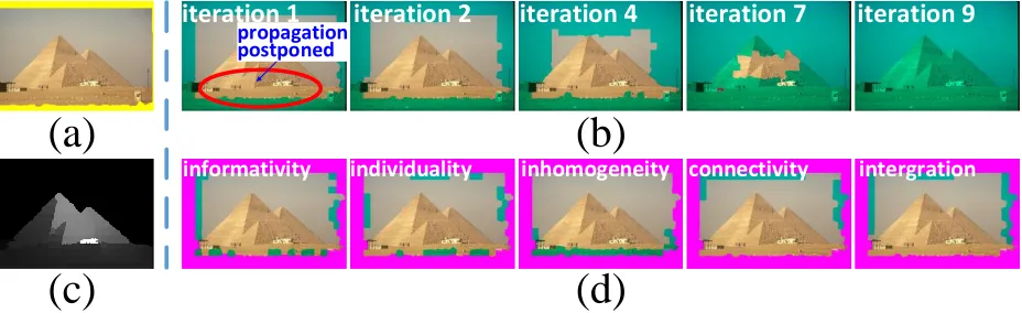
Figure 5: Visualization of the designed propagation process. (a) shows the input image with boundary seeds (yellow). (b) displays the propagations in several key iterations, and the expansions of labeled setLare highlighted with light green masks. (c) is the final saliency map. The curriculum superpixels of the 2nd iteration decided by informativity, individuality, inhomogeneity, connectivity, and the final integrated result are visualized in (d), in which the magenta patches represent the learned superpixels in the 1st propagation, and the regions for the 2nd diffusion are annotated with light green.

5(a)). In (b), we observe that the sky regions are relatively easy and are firstly learned during the 1st∼4th iterations. In contrast, the land areas are very different from the seeds, so they are difficult and their diffusion should be deferred. Though the labeled set touches the land in a very early time (see the red circle in the 1st iteration), the land superpixels are not diffused until the 4th iteration. This is because the background regions are mostly learned until the 4th iteration, which provide sufficient preliminary knowledge to identify the difficult land regions as foreground or background. As a result, the learner is more confident to assign the correct saliency values to the land after the 4th iteration, and the target (pyramid) is learned in the end during the 7th∼9th iterations. More concretely, the effect of our curriculum selection approach is demonstrated in Fig.5(d). It can be observed that though the curriculum superpixels are differently chosen by their informativity, individuality, inhomogeneity, and connectivity, they are easy to learn based on the previous accumulated knowledge. Particularly, we notice that the final integrated result only preserves the sky regions for the leaner, while discards the land areas though they are recommended by informativity, individuality, and inhomogeneity. This further reduces the erroneous propagation possibility since the land looks differently from the sky and actually more similar to the unlearned pyramid. Therefore, the fusion scheme (3.1) and the properq(t)decided by the learning-to-teach step are reasonable and they are critical to the successful propagations (see Fig.5(c)).

4

Physical Interpretation and Justification

A key factor to the effectiveness of our method is the well-ordered learning sequence from simple to difficult, which is also considered by curriculum learning [2] and self-paced learning [15]. This paper introduces this strategy to graph-based saliency propagation. More interestingly, we provide a physical interpretation of this strategy, by relating the curriculum guided propagation to the practical fluid diffusion.

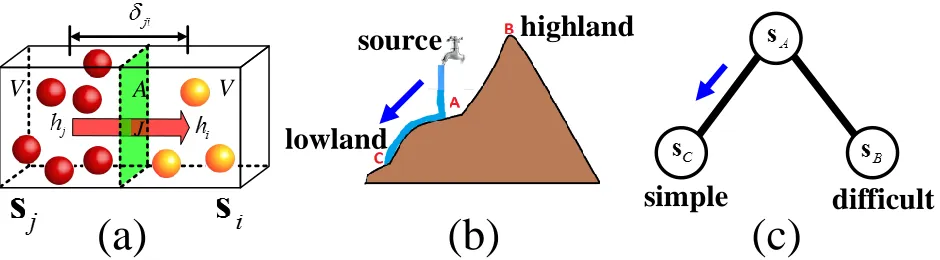
In physics,Fick’s Law of Diffusion[6] is well-known for understanding the mass transfer of solids, liquids, and gases through diffusive means. It postulates that the flux diffuses from regions of high concentration to regions of low concentration, with a magnitude that is proportional to the concentration gradient (see Fig.6(a)). Along one diffusive direction, the law is formulated as

J=−γ∂h

∂δ, (4.1)

whereγis the diffusion coefficient,δ is the diffusion distance,his the concentration that evaluates the density of molecules of fluid, andJ is the diffusion flux that measures the quantity of molecules flowing through the unit area per unit time.

A

J

V

V

(a)

(b)

(c)

simple

difficult

highland

lowland

source

Figure 6: The physical interpretation of our saliency propagation algorithm. (a) analogies the propagation between two regions with equal difficulty to the fluid diffusion between two cubes with same altitude. The left cube with more balls is compared to the region with larger saliency value. The right cube with fewer balls is compared to the region with less saliency cues. The red arrow indicates the diffusion direction. (b) and (c) draw the parallel between fluid diffusion with different altitudes and saliency propagation guided by curriculums. The lowland “C”, highland “B”, and source “A” in (b) correspond to the simple nodesC, difficult nodesB, and labeled nodesAin (c), respectively.

Like the fluid can only flow from “A” to the lowland “C” in (b),sAin (c) also tends to transfer the saliency value to

the simple nodesC.

cannot be transmitted from lowlands to highlands. Therefore, by treatingγas the propagation coefficient,has the saliency value (equivalent tof in above sections), andδas the propagation distance defined byδji= 1/

√

ωji, (4.1)

explains the process of saliency propagation fromsjtosias

Jji=−miγ

f_i(t)−f_j(t) δji

=−miγ

√

ωji(f

(t)

i −f

(t)

j ). (4.2)

The parametermi in (4.2), which plays the same role asMiiin (3.12), denotes the “altitude” ofsi. It equals to

1 ifsicorresponds to a lowland, and 0 ifsi represents a highland. Note that ifsi is higher thansj, the fluxJji = 0

because the fluid cannot transfer from lowland to highland. Given (4.2), we have the following theorem:

Theorem 1: Suppose all the superpixelss1,· · ·,sN in an image are modelled as cubes with volumeV, and the area

of their interface isA. By usingmi to indicate the altitude ofsi and setting the propagation coefficientγ = 1, the

proposed saliency propagation can be derived from the fluid transmission modelled by Fick’s Law of Diffusion. We put the detailed proof in thesupplementary materialdue to the limited page length. Theorem 1 reveals that our propagation method can be perfectly explained by the well-known physical theory.

5

Experimental Results

In this section, we qualitatively and quantitatively compare the proposedTeaching-to-Learn andLearning-to-Teach approach (abbreviated as “TLLT”) with twelve popular methods on two popular saliency datasets. The twelve baselines include classical methods (LD [18], GS [24]), state-of-the-art methods (SS [8], PD [19], CT [14], RBD [30], HS [25], SF [22]), and representative propagation based methods (MR [27], GP [7], AM [12], GRD [26]). The parameters in our method are set toN= 400andθ= 0.25throughout the experiments.

5.1

Metrics

Margolinet al. [20] point out that the traditional Precision-Recall curve (PR curve) andFβ-measure suffer the

inter-polation flaw, dependency flaw and equal-importance flaw. Instead, they propose the weighted precision Precisionw_,

weighted recall Recallw and weightedFβ-measureFβw to achieve more reasonable evaluations. In this paper, we

adopt this recently proposed metrics [20] to evaluate the algorithms’ performance. The parameter β2 in F_βw = (1 +β2₎ Precisionw_+Recallw

β2_Precisionw_+Recallw is set to 0.3 as usual to emphasize the precision [27,25]. Fig. 7shows some examples

0.736

0.797

0.955

0.906

(b)

(c)

(a)

Figure 7: The comparison of traditional PR curve vs. the metric in [20]. (a) shows two saliency maps generated by MR [27] and our method. The columns are (from Left to Right): input images, MR results, our results, and groundtruth. (b), (c) present the PR curves over the images in the first and second rows of (a), respectively. In the top image of (a), our more confident result surprisingly receives the similar evaluation with MR reflected by (b). In the bottom image, the MR result fails to supress the flowers in the background, but turns out to be significantly better than our method revealed by (c). In contrast, the weightedFβ-measureFβw(light blue numbers in (a)) provides more reasonable

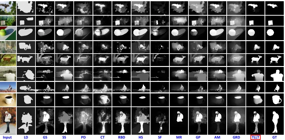
Input LD GS SS PD CT RBD HS SF MR GP AM GRD TLLT GT

Figure 8: Visual comparisons of saliency maps generated by all the methods on some challenging images. The ground truth (GT) is presented in the last column.

Table 1: Average CPU seconds of all the approaches on ECSSD dataset

Method LD GS SS PD CT RBD HS SF MR GP AM GRD TLLT

Duration (s) 7.24 0.18 3.58 2.87 3.53 0.20 0.43 0.19 0.87 3.22 0.15 0.93 2.05 Code matlab matlab matlab matlab matlab matlab C++ matlab matlab matlab matlab matlab matlab

5.2

Experiments on Public Datasets

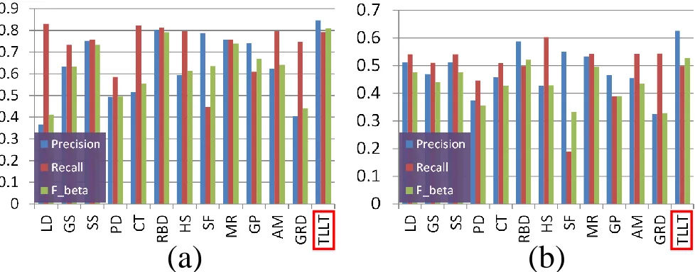
The MSRA 1000 dataset [18], which contains 1000 images with binary pixel-level groundtruth, is firstly adopted for our experiments. The average precisionw, recallw, andFw

β of all the methods are illustrated in Fig. 9(a). We

can observe that the Fw

β of our TLLT is larger than 0.8, which is the highest record among all the comparators.

Another notable fact is that TLLT outperforms other baselines with a large margin in Precisionw. This is because the designed teaching-to-learn and learning-to-teach paradigm propagates the saliency value carefully and accurately. As a result, our approach has less possibility to generate the blurred saliency map with confused foreground. In this way, the Precisionw_{is significantly improved. More importantly, we note that the Recall}w _{of our method also touches a}

relatively high value, although the Precisionw_{has already obtained an impressive record. This further demonstrates}

the strength of our innovation.

Although the images from MSRA 1000 dataset have a large variety in their content, the foreground is actually prominent among the simple and structured background. Therefore, a more complicated dataset ECSSD [25], which represents more general situations that natural images fall into, is adopted to further test all the algorithms. Fig. 9(b) shows the result. Generally, all methods perform more poorly on ECSSD than on the MSRA 1000. However, our algorithm still achieves the highestF_βwand Precisionw when compared with other baselines. RBD obtains slightly lowerF_βwthan our method with 0.5215 compared to 0.5283, but the weighted precision is not as good as our approach. Besides, some methods that show very encouraging performance under the traditional PR curve metric, such as HS, SF and GRD, only obtain very moderate results under the new metrics. Since they tend to detect the most salient regions at the expense of low precision, the imbalance between Precisionw and Recallw will happen, which pulls down the overallFw

β to a low value. Comparatively, TLLT produces relatively balanced Precision

w_{and Recall}w

on both datasets, therefore higherFw

β is obtained.

(a)

(b)

Figure 9: Comparison of different methods on two saliency detection datasets. (a) is MSRA 1000, and (b) is ECSSD.

suitable curriculum in every iteration, it needs relatively longer computational time. The iteration times for a normal image under our parametric settings are usually 5∼15. However, better results can be obtained as shown in Fig. 9, at the cost of more computational time.

To further present the merits of the proposed approach, we provide the resulting saliency maps of evaluated meth-ods on several very challenging images from the two datasets (see Fig. 8). Though the backgrounds in these images are highly complicated, or very similar to the foregrounds, TLLT is able to generate fairly confident and clean saliency maps. In other words, TLLT is not easily confused by the unstructured background, and can make a clear distinction between the complex background and the regions of interest.

5.3

Parametric Sensitivity

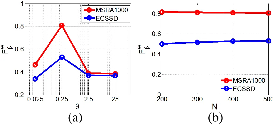
There are two free parameters in our algorithm to be manually tuned: Gaussian kernel widthθ and the amount of superpixelsN. We evaluate each of the parametersθ andN by examiningF_βw with the other one fixed. Fig. 10

reveals thatFw

β is not sensitive to the change ofN, but heavily depends on the choice ofθ. Specifically, it can be

observed that the highest records are obtained whenθ = 0.25on both datasets, so we adjustθ to 0.25 for all the experiments.

6

Conclusion

This paper proposed a novel approach for saliency propagation through leveraging a teaching-to-learn and learning-to-teach paradigm. Different from the existing methods that propagated the saliency information entirely depending on the relationships among adjacent image regions, the proposed approach manipulated the propagation sequence from simple regions to difficult regions, thus leading to more reliable propagations. Consequently, our approach can render a more confident saliency map with higher background suppression, yielding a better popping out of objects of interest. Our approach is inspired by the theoretical results in educational psychology, and can also be understood from the well-known physical diffusion laws. Future work may study accelerating the proposed method and meanwhile exploring more insightful learning-to-teach principles.

References

(a)

(b)

Figure 10: Parametric sensitivity analyses: (a) shows the variation ofF_βww.r.t.θby fixingN = 400; (b) presents the change ofF_βww.r.t.N by keepingθ= 0.25.

[2] Y. Bengio, J. Louradour, R. Collobert, and J. Weston. Curriculum learning. InProc. International Conference on Machine Learning, pages 41–48. ACM, 2009.

[3] C. Bishop. Pattern recognition and machine learning, volume 1. springer New York, 2006.

[4] M. Cheng, G. Zhang, N. Mitra, X. Huang, and S. Hu. Global contrast based salient region detection. InComputer Vision and Pattern Recognition (CVPR), IEEE Conference on, pages 409–416. IEEE, 2011.

[5] J. Elman. Learning and development in neural networks: The importance of starting small.Cognition, 48(1):71– 99, 1993.

[6] A. Fick. On liquid diffusion. The London, Edinburgh, and Dublin Philosophical Magazine and Journal of Science, 10(63):30–39, 1855.

[7] K. Fu, C. Gong, I. Gu, and J. Yang. Geodesic saliency propagation for image salient region detection. InImage Processing (ICIP), IEEE Conference on, pages 3278–3282, 2013.

[8] K. Fu, C. Gong, I. Gu, J. Yang, and X. He. Spectral salient object detection. InMultimedia and Expo (ICME), IEEE International Conference on, 2014.

[9] V. Gopalakrishnan, Y. Hu, and D. Rajan. Random walks on graphs to model saliency in images. InComputer Vision and Pattern Recognition (CVPR), IEEE Conference on, pages 1698–1705. IEEE, 2009.

[10] X. Hou and L. Zhang. Saliency detection: A spectral residual approach. In Computer Vision and Pattern Recognition (CVPR), IEEE Conference on, pages 1–8. IEEE, 2007.

[11] L. Itti, C. Koch, and E. Niebur. A model of saliency-based visual attention for rapid scene analysis. Pattern Analysis and Machine Intelligence, IEEE Transactions on, 20(11):1254–1259, 1998.

[12] B. Jiang, L. Zhang, H. Lu, C. Yang, and M. Yang. Saliency detection via absorbing markov chain. InComputer Vision (ICCV), IEEE International Conference on, pages 1665–1672. IEEE, 2013.

[13] F. Khan, B. Mutlu, and X. Zhu. How do humans teach: On curriculum learning and teaching dimension. In

Advances in Neural Information Processing Systems, pages 1449–1457, 2011.

[14] J. Kim, D. Han, Y. Tai, and J. Kim. Salient region detection via high-dimensional color transform. InComputer Vision and Pattern Recognition (CVPR), IEEE Conference on, pages 883–890. IEEE, 2014.

[15] M. Kumar, B. Packer, and D. Koller. Self-paced learning for latent variable models. InAdvances in Neural Information Processing Systems, pages 1189–1197, 2010.

[17] Y. Li, X. Hou, C. Koch, J. Rehg, and A. Yuille. The secrets of salient object segmentation. InComputer Vision and Pattern Recognition (CVPR), IEEE Conference on, pages 280–287. IEEE, 2014.

[18] T. Liu, J. Sun, N. Zheng, X. Tang, and H. Shum. Learning to detect a salient object. InComputer Vision and Pattern Recognition (CVPR), IEEE Conference on, pages 1–8. IEEE, 2007.

[19] R. Margolin, A. Tal, and L. Zelnik-Manor. What makes a patch distinct? In Computer Vision and Pattern Recognition (CVPR), IEEE Conference on, pages 1139–1146. IEEE, 2013.

[20] R. Margolin, L. Zelnik-Manor, and A. Tal. How to evaluate foreground maps. InComputer Vision and Pattern Recognition (CVPR), IEEE Conference on, pages 248–255. IEEE, 2014.

[21] S. Maybank. A probabilistic definition of salient regions for image matching. Nuerocomputing, 120(23):4–14, 2013.

[22] F. Perazzi, P. Krahenbuhl, Y. Pritch, and A. Hornung. Saliency filters: Contrast based filtering for salient region detection. InComputer Vision and Pattern Recognition (CVPR), IEEE Conference on, pages 733–740. IEEE, 2012.

[23] D. Rohde and D. Plaut. Language acquisition in the absence of explicit negative evidence: How important is starting small? Cognition, 72(1):67–109, 1999.

[24] Y. Wei, F. Wen, W. Zhu, and J. Sun. Geodesic saliency using background priors. InEuropean Conference on Computer Vision (ECCV), pages 29–42. Springer, 2012.

[25] W. Yan, L. Xu, J. Shi, and J. Jia. Hierarchical saliency detection. InComputer Vision and Pattern Recognition (CVPR), IEEE Conference on, pages 1155–1162. IEEE, 2013.

[26] C. Yang, L. Zhang, and H. Lu. Graph-regularized saliency detection with convex-hull-based center prior.Signal Processing Letters, IEEE, 20(7):637–640, 2013.

[27] C. Yang, L. Zhang, H. Lu, X. Ruan, and M. Yang. Saliency detection via graph-based manifold ranking. In

Computer Vision and Pattern Recognition (CVPR), IEEE Conference on, pages 3166–3173. IEEE, 2013. [28] J. Yang and M. Yang. Top-down visual saliency via joint CRF and dictionary learning. InComputer Vision and

Pattern Recognition (CVPR), IEEE Conference on, pages 2296–2303. IEEE, 2012.

[29] D. Zhou, J. Weston, A. Gretton, O. Bousquet, and B. Sch¨olkopf. Ranking on data manifolds.Advances in Neural Information Processing Systems, 16:169–176, 2004.

[30] W. Zhu, S. Liang, Y. Wei, and J. Sun. Saliency optimization from robust background detection. InComputer Vision and Pattern Recognition (CVPR), IEEE Conference on, pages 2814–2821. IEEE, 2014.