Tractable interval temporal propositional and description logics

BIROn - Birkbeck Institutional Research Online

Artale, A. and Kontchakov, Roman and Ryzhikov, V. and Zakharyaschev,

Michael (2015) Tractable interval temporal propositional and description

logics. In: UNSPECIFIED (ed.) Proceedings of the 29th AAAI Conference

on Artificial Intelligence, AAAI-15. AAAI, pp. 1417-1423.

Downloaded from:

Usage Guidelines:

Please refer to usage guidelines at

or alternatively

Tractable Interval Temporal Propositional and Description Logics

A. Artale

_and

_{R. Kontchakov}

_and

_{V. Ryzhikov}

_and

_{M. Zakharyaschev}

Free University of Bozen-Bolzano, Italy Birkbeck, University of London, U.K.

{artale,ryzhikov}@inf.unibz.it {roman,michael}@dcs.bbk.ac.uk

Abstract

We design a tractable Horn fragment of the Halpern-Shoham temporal logic and extend it to interval-based temporal de-scription logics, instance checking in which is P-complete for both combined and data complexity.

Introduction

The aims of this paper are to (i) design a tractable sub-Boolean fragment of the Halpern-Shoham interval temporal logicHS(Halpern and Shoham 1991) and (ii) construct on its basis tractable descriptions logics with temporal interval operators. The design of these logics is motivated by possi-ble applications in ontology-based data access over temporal databases (which will be discussed at the end of the paper).

The Halpern-Shoham logicHSis an extension of proposi-tional logic with temporal operators of the formhRi, whereR

is one of Allen’s (1981) interval relations (after,begins,ends,

during,later,overlaps,equalsand their inverses). The propo-sitional variables ofHS are interpreted by sets of closed intervals[i, j]of some flow of time (such as_Z,_R, etc.), and a formulahRiϕis regarded to be true in[i, j]iffϕis true in some interval[i0, j0]such that[i, j]R[i0, j0]in Allen’s in-terval algebra. Unfortunately, this natural and seemingly simple logic turned out to be highly undecidable (Halpern and Shoham 1991). One explanation of the bad computa-tional behaviour ofHS is that it can be viewed as a two-dimensional modal logic interpreted over products of (linear) Kripke frames, which provide a good playground for sim-ulating Turing machines, tilings, lossy channels, etc.; see, e.g., (Marx and Venema 1997; Marx and Reynolds 1999; Reynolds and Zakharyaschev 2001; Gabelaia et al. 2005; Konev, Wolter, and Zakharyaschev 2005; Gabelaia et al. 2006; Hampson and Kurucz 2014).

The interest in interval temporal logics was renewed in the 2000s when decidable fragments of HS were con-structed by restricting the available sets of temporal op-erators (Bresolin et al. 2009). The reader can check the current decidability status of numerous fragments of HS

over various time-lines atitl.dimi.uniud.it/content/logic-hs; see also (Lodaya 2000; Bresolin et al. 2012b; 2012a; 2014a; Marcinkowski and Michaliszyn 2014; Bresolin et al. 2014b;

Copyright c2015, Association for the Advancement of Artificial Intelligence (www.aaai.org). All rights reserved.

Montanari, Puppis, and Sala 2014) and references therein. The computational complexity of the decidable fragments ranges from NP to EXPSPACEover strongly discrete linear orders, and from NP to non-primitive recursive over finite lin-ear orders. Bresolin, Mu˜noz-Velasco, and Sciavicco (2014) defined a ‘Horn fragment’ of HS; alas, overZand other

strongly discrete linear orders, it turned out to be undecid-able.

In this paper, we consider a somewhat different Horn frag-ment, denotedHShorn, which comprises formulasϕgiven by

the following grammar:

λ ::= p | hRiλ | [R]λ, λ+ ::= p | [R]λ+, ψ ::= λ1∧ · · · ∧λk→λ+ | λ1∧ · · · ∧λk→ ⊥,

ϕ ::= p[m, n] | [G]ψ | ϕ1∧ϕ2,

wherepis a propositional variable,Rany interval relation,

[R]the dual of hRi, and[G]the universal modality ‘in all intervals’. Formulas of the formp[m, n]areinitial clauses

(data) stating thatpholds in the interval[m, n]; formulas of the form[G]ψareuniversal clausesdescribing general transformation rules and constraints; cf. (Fisher, Dixon, and Peim 2001). Our first result is that the satisfiability problem forHShornover the flow of timeZis P-complete (for both

combined and data complexity) provided that the interpreta-tion of the interval relainterpreta-tions isnon-strict(e.g.,[i, j]L[i0, j0]

iffj≤i0—rather thanj < i0), which corresponds to the se-mantics of SQL:2011. Under the strict interpretation,HShorn

becomes PSPACE-hard. Note that the right-hand side of the implicationsψcan only use ‘boxes’[R]. If ‘diamonds’hRi

were also allowed, then the resulting fragment would be un-decidable, as easily follows from the undecidability result of Bresolin, Mu˜noz-Velasco, and Sciavicco (2014).

Having identified a tractable fragment of HS, we can use it as a template to define (hopefully tractable) temporal ontology languages. In this paper, we construct a temporali-sationHS-LiteHhornof the description logicDL-Lite

H

horn

(Cal-vanese et al. 2007; Artale et al. 2009), which is a Horn ex-tension of the ontology-based data access standard language OWL 2 QL1_{. InHS-Lite}H

horn, we represent temporal data by

means of assertions such as

SummerSchool(RW, t1, t2), teaches(RK,DL, s1, s2),

1

www.w3.org/TR/owl2-profiles/#OWL 2 QL

which say that RW is a summer school that takes place in the time interval[t1, t2]and RK teaches DL in[s1, s2]. Note that

temporal databases store data in a similar format (Kulkarni and Michels 2012). Temporal concept and role inclusions are used to impose various constraints on the data and introduce new concepts and roles. For example, according to

h_D¯_{iMorningSessionuAdvancedCoursev ⊥,}

advanced courses cannot be given during the morning ses-sions; the axiom

hB¯iLectureDayu hAiLunchvMorningSession

‘defines’ morning sessions (note that we are not allowed to replacevwith≡in this axiom). The inclusion

teachesv[D]teaches

claims that the roleteachesis downward hereditary (or sta-tive) in the sense that if it holds in some interval, then it also holds in all of its sub-intervals. If, instead, we want to state thatteachesis coalesced (or upward hereditary), in the sense thatteachesholds in any interval covered by sub-intervals where it holds, then we can use

[D](hOiteachest h_D¯_iteaches)u

hBiteachesu hEiteachesvteaches. By removing the last two conjuncts on the left-hand side of this axiom, we make sure thatteachesis both upward and downward hereditary. For a discussion of these notions in temporal databases, consult (B¨ohlen, Snodgrass, and Soo 1996; Terenziani and Snodgrass 2004).

Although the complexity of fullHS-LiteH_hornremains un-known, in this paper we define two interesting fragments, for which instance checking is P-complete for both com-bined and data complexity. One fragment, HS-LiteH_horn[G], restricts the use of temporal operators in role inclusion ax-ioms, where only the ‘universal’[G]is allowed. The second one,HS-LiteH_horn/flat, allows only atomic concepts on the right-hand side of concept inclusions (but does not impose any restrictions on role inclusions).

The omitted proofs are available in (Artale et al. 2015).

Tractable

HS

The syntax of the logicHShornwas defied in the introduction.

In this paper, we consider the interval relationsA,A,¯ B,B,¯ E,E,¯ D,D,¯ L,L,¯ O,O¯andGover the set of closed intervals

[i, j] ={n∈Z|i≤n≤j}, for any integer numbersi≤j,

defined by taking:

– [i, j]A[i0, j0] iff j =i0, (After) – [i, j]B[i0_{, j}0_{] iff i=i}0_andj≥j0_{, (Begins)}

– [i, j]E[i0_{, j}0_{] iff i≤i}0_andj=j0_{, (Ends)}

– [i, j]D[i0, j0] iff i≤i0andj ≥j0, (During) – [i, j]L[i0, j0] iff j≤i0, (Later) – [i, j]O[i0, j0] iff i≤i0 ≤jandj ≤j0, (Overlaps) andA,¯ B,¯ E,¯ D,¯ L,¯ O¯to be the inverses ofA,B,E,D,L, O, respectively. Note that we allow single-point intervals

[i, i]and use non-strict≤instead of the more common<.

p

h_B¯_ip

h_E¯_ip

q

hBiq

hEiq

i j

p

h_A¯_ip

hAip

i j

Figure 1: Semantics of the temporal operators: intervals[i, j]

are shown as points with the coordinates(i, j)and, e.g., ifp is true in[−1,1]thenh_E¯_{ipis true in all[−k,1], fork≤ −1.}

Example 1. Consider the followingHShorn-formula

ϕ = p[−1,0]∧q[0,0]∧q[0,3]∧

[G](hEip→q)∧[G]([ ¯A]q∧q→r). The first three conjuncts—p[−1,0],q[0,0]andq[0,3]—are calledinitial clauses: they state thatpholds in[−1,0]and qin[0,0]and[0,3]. The numbers occurring in the initial conditions are calledtemporal constantsand given in binary.

Aninterpretation,M, forHShornassigns to every interval [i, j]inZa set of propositional variables,p, that are regarded

to betruein[i, j], in which case we writeM,[i, j]|=p. This truth-relation is extended toHShorn-formulas by taking:

– M,[i, j]|=p[m, n] iff M,[m, n]|=p,

– M,[i, j]|=hRiα iff M,[i0, j0]|=αfor some interval

[i0, j0]such that[i, j]R[i0, j0], – M,[i, j]|= [R]α iff M,[i0, j0]|=αfor all intervals

[i0_{, j}0_{]such that[i, j]R[i}0_{, j}0_],

and the usual clauses for the Booleans; see Fig. 1. AnHShorn

-formulaϕissatisfiableif there is an interpretationMsuch thatM,[0,0] |= ϕ; in this case we call Mamodelofϕ and writeM|=ϕ. The length ofϕis denoted by|ϕ|. Our main result in this section is a polynomial-time algorithm for checking satisfiability ofHShorn-formulas (this problem is

P-hard as the language contains propositional Horn clauses). We represent any HShorn-formulaϕas Ξ∧Ψ+ ∧Ψ−,

whereΞis a conjunction of the initial clauses inϕandΨ+

(respectively,Ψ−) is a conjunction of the universal clauses

[G]ψinϕwithλ+_{(respectively,⊥) on the right-hand side.}

Lemma 2. AnyHShorn-formula can be transformed in

poly-nomial time to an equisatisfiable formulaΞ∧Ψ+∧Ψ−such that it does not contain diamond operators, and its box oper-ators only occur in contexts of the form[G]ψand[R]p, where R∈ {A,A, B,¯ B, E,¯ E, G¯ }andpa propositional variable.

Proof. First, we express every[R]λandhRiλin terms of the operators mentioned above: for instance,[D]pis equivalent to[B][E]p(see also Fig. 1). Then we replace every nestedλ with a fresh variablepλand add[G](λ→pλ)as a conjunct;

we also replace every nestedλ+ _{with a freshp}

λ+ and add [G](pλ+ → λ+). Finally, we eliminate the diamonds by

Figure 2: Partition ofZwith respect to{−1,0,3}.

From now on we only considerHShorn-formulas of the

formϕ= Ξ∧Ψ+_∧Ψ−_{given by Lemma 2. We now define}

acanonical(orminimal)interpretationKϕforϕby taking,

for any variablepand any interval[i, j],

Kϕ,[i, j]|=p iff M,[i, j]|=p for allM|= Ξ∧Ψ+.

Clearly,Ξ∧Ψ+is always satisfiable.

Lemma 3. For any formulaϕ= Ξ∧Ψ+_∧Ψ−_{, we have} Kϕ|= Ξ∧Ψ+. Moreover,ϕis satisfiable iffKϕ|=ϕ.

Note that the Horn fragment ofHSdefined by (Bresolin, Mu˜noz-Velasco, and Sciavicco 2014) does not enjoy this min-imal model property becausehRion the right-hand side can represent disjunction; see (Artale et al. 2007, Theorem 11).

We now show how to construct efficiently the canonical interpretation for a given formula. We will require the fol-lowing notation. LetZω=Z∪ {−ω, ω}with−ω < i < ω,

for any i ∈ Z. Given i, j ∈ Zω, for i ≤ j, we set (i, j) = {n ∈ _Z | i < n < j}. For a non-empty subset M ={m0, m1, . . . , mn}ofZwithm0< m1<· · ·< mn,

we define thepartition ofZwith respect toM to be the set IM comprising the following intervals:

– (−ω, m0),(mn, ω)and[mk, mk], for0≤k≤n;

– (mk, mk+1), for(mk, mk+1)6=∅and0≤k < n.

IfM =∅, we set_IM ={(−ω, ω)}. Note thatI∩I0 =∅, for any distinctI, I0∈IM, andSI∈IMI=Z.

Given a formulaϕ= Ξ∧Ψ+_∧Ψ−_{, we denote byM}

ϕthe

set of integers occurring inΞ. Note that|IMϕ|is linear in|ϕ|:

for instance, forϕfrom Example 1,Mϕ={−1,0,3}and

IMϕ={(−ω,−1),[−1,−1],[0,0],(0,3),[3,3],(3, ω)},

see Fig. 2. The following lemma provides a key to the struc-ture of canonical interpretations:

Lemma 4. Letϕbe anHShorn-formula,pa variable and

I, J ∈IMϕ. If there existi ∈Iandj ∈J withi≤jand

Kϕ,[i, j]|=p, thenKϕ,[i0, j0]|=pfor alli0 ∈Iandj0∈J

withi0≤j0.

This lemma shows that the canonical interpretation for ϕcan be constructed by applying the rules in Ψ+ _{to the}

closed intervals in thefinitelinear order(IMϕ,), where

is defined by takingI J, forI, J ∈ _IM, iffi ≤ j, for somei∈Iandj∈J. The interval relations[I, J]R[I0, J0]

in(IMϕ,), forR∈ {A,A, B,¯ B, E,¯ E, G¯ }, are defined as

usual. Now, the canonical interpretation forϕ= Ξ∧Ψ+∧Ψ−

can be constructed using the followingchase procedure. We first setCϕ={(p,[m, m],[n, n]) |p[m, n]∈Ξ}and then

apply toCϕthe following rules: Suppose(pk, I, J) ∈Cϕ,

for1 ≤k≤h, and(qk, I0, J0)∈Cϕ, for allI0, J0 ∈IMϕ

with[I, J]Rk[I0, J0]and1≤k≤`, then

– Ifp1∧ · · · ∧ph∧[R1]q1∧ · · · ∧[R`]q`→pis inΨ+then

Cϕ:=Cϕ∪ {(p, I, J)}.

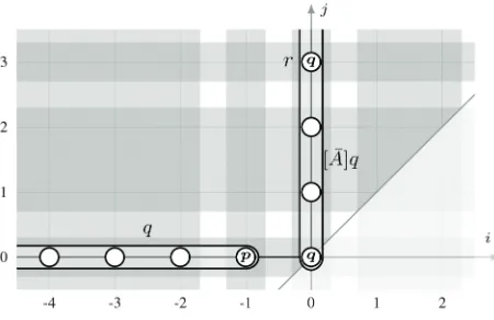
Figure 3: Canonical interpretation from Example 5.

– Ifp1∧ · · · ∧ph∧[R1]q1∧ · · · ∧[R`]q` →[R]pis inΨ+

thenCϕ:=Cϕ∪ {(p, I0, J0)|[I, J]R[I0, J0]}.

AsCϕ⊆Vϕ×IMϕ×IMϕ, whereVϕis the set of variables

inϕ, and|IMϕ| = O(|ϕ|), the chase procedure reaches a

fixed pointC∗_ϕafterpolynomially manysteps. The canonical interpretationKϕis now defined by takingKϕ,[i, j]|=piff (p, I, J)∈C∗_ϕ,i∈Iandj∈J.

Example 5. The canonical interpretation Kϕ for ϕfrom

Example 1 can be defined by taking (see Fig. 3):

Kϕ,[i, j]|=p iff i=−1, j= 0,

Kϕ,[i, j]|=q iff i≤0, j= 0 or i= 0, j= 3,

Kϕ,[i, j]|=r iff i= 0, j= 0 or i= 0, j= 3.

As a consequence of the (polynomial) construction of the canonical interpretations and Lemma 3, we obtain:

Theorem 6. The satisfiability problem forHShorn-formulas

isP-complete.

Another consequence of the construction (which will be used in the proof of Lemma 13) is that satisfiability ofHShorn

-formulas is preserved under the following scaling of initial clauses. Letϕi= Ξi∧Ψ+∧Ψ−andMϕi ={m

i

0, . . . , min}

withmi

0 <· · ·< min, fori= 1,2. We say thatϕ1andϕ2

arevariantsif

– min{m1_k+1 −m1_k,2} = min{m2_k+1−m2_k,2}, for any

0≤k < n, – p[m1

i, m1j]∈Ξ1iffp[m2i, m2j]∈Ξ2, for any variablep.

The former condition means that the difference between the adjacentmi

kis the same for bothimodulo counting in terms

of 0, 1 andmany. It follows, in particular, that(IMϕ1,)and (IMϕ2,)are isomorphic as linear orders (see also

Exam-ple 8). The two conditions together imply the following:

Lemma 7. Any two variants are equisatisfiable.

Remark 9. If in place of≤in the definition of the interval relations we take<, then reasoning withHShornbecomes

non-tractable (unless P = PSPACE). Indeed, given a Tur-ing machineAwith polynomial tape, we take the following initial clauses: ai[0,0] to say that input celli containsa,

h0[0,0]to indicate that the head scans the left-most cell,

andq0[0,0]to fix the initial stateq0. Instructions such as (q, a)→(q0, a0, R)are encoded by formulas of the form

[G] hE¯i[B](q∧ai∧hi)→q0∧a0i∧hi+1.

(Thus, we represent the consecutive configurations ofAon the ‘diagonal intervals’[n, n],n ≥0, using the ‘previous-time’ operator hE¯i[B].) ThenAaccepts the input iff the conjunction of the above formulas and[G](q1 → ⊥), for

the accepting stateq1, is unsatisfiable. At the moment, the

exact complexity ofHShornunder the strict semantics is not

known. Note that the fullEB-fragment of¯ HS is undecid-able (Bresolin et al. 2014a).

Data Complexity

AsHShorn-formulas consist of initial clauses (that is,data)

and universal clauses, we can also measure the complexity of the satisfiability problem in terms of the size of the data regarding the universal clauses fixed.

Theorem 10. HShornisP-complete for data complexity.

Proof. Theorem 6 gives the upper bound. The proof of hardness is by a LOGSPACE-reduction of the monotone

cir-cuit value problem, which is known to be P-complete; see e.g., (Greenlaw, Hoover, and Ruzzo 1995; Miyano, Shiraishi, and Shoudai 1990). SupposeCis a monotone circuit whose vertices (sources, gates and sink) are enumerated by con-secutive positive integers in such a way that if there is an edge from a vertexnto a vertexm—in which case we write n;m—thenn < m. Denote bymaxCthe maximum of the vertex numbers. We can assume thatmaxCis the sink ofC (somaxC−1 ;maxC). We representC(~x), for an input~x, by the conjunctionΞC(~x)of the following initial

clauses:

– t[maxC−1,maxC],

– t[n, m] (orf[n, m]) ifnis a source with input value 1 (respectively, 0) andn;m;

– AND[n, m](or OR[n, m]) ifnis an AND gate (respec-tively, OR gate) andn;m;

– and[0, m]andt[n, m], for eachnsuch that0 < n≤ m andn6;m, ifmis an AND gate;

– or[0, m]andf[n, m], for eachnsuch that0< n≤mand n6;m, ifmis an OR gate.

LetΨ+_{be a conjunction of the following universal clauses:} [G](hA¯if∧AND→f), [G]([ ¯A]f∧OR→f),

[G]([ ¯A]t∧AND→t), [G](hA¯it∧OR→t),

[G](and→[ ¯E]t), [G](or→[ ¯E]f),

and letΨ− = [G](t∧f → ⊥). It is not hard to check that

ΞC(~x)∧Ψ+∧Ψ−is satisfiable iffC(~x) = 1. (Intuitively,

the last items in the definitions of the initial and universal

clauses ensure that, for any OR gatem, all intervals of the form[n, m]withn6;mare labelled withf; and dually the AND gates witht. Thus, the output of any gate only depends

on its inputs.) _q

It is of interest to note that a similar Horn fragment of the point-basedLTL is in AC0for data complexity, while the wholeLTL is NC1-complete (Artale et al. 2014a); we remind the reader that AC0$NC1⊆P.

We now useHShornas a template for defining a

tempo-ral extension of the description logicDL-LiteH_hornwith the ultimate aim of employing it or its suitable fragments for ontology-based data access over temporal databases.

Description Logic

HS

-Lite

The language of HS-LiteH_horn contains individual names

a0, a1, . . ., concept names A0, A1, . . ., and role names

P0, P1, . . ..Basic rolesR,basic conceptsB,temporal roles

Sandtemporal conceptsCare given by the following gram-mar:

R ::= Pk | P_k−, B ::= Ak | ∃R,

S ::= R | [R]S, C ::= B | [R]C, whereR is one of the interval relations. An HS-LiteH_horn

TBox is a finite set ofconceptandrole inclusions

C1u · · · uCkvC, S1u · · · uSk vS,

anddisjointness constraints

C1u · · · uCk v ⊥, S1u · · · uSkv ⊥.

Note that, similarly to Lemma 2, we could also allow the diamond operatorshRiCandhRiSon theleft-hand sideof concept and role inclusions and disjointness constraints. They are omitted to simplify presentation.

AnHS-LiteHhornABox is a finite set of atoms of the form

Ak(a, i, j) and Pk(a, b, i, j) in which temporal constants

i≤jare given in binary. The set of individual names inA

is denoted byind(A). AnHS-LiteH_hornknowledge base(KB) is a pairK= (T,A), whereT is a TBox andAan ABox.

An HS-LiteH_horn interpretation, I, consists of a family of standard (atemporal) description logic interpretations

I[i, j] = (∆I_,·I[i,j]_{), for alli, j ∈}

Zwithi≤j, in which ∆I 6=∅,aI[i,j]

k =aIk for some (fixed)aIk ∈∆I,⊥I[i,j]=∅,

AI[i,j]

k ⊆∆IandPkI[i,j] ⊆∆I×∆I. The role and concept

constructs are interpreted inIas follows:

(P_k−)I[i,j] = {(x, y)|(y, x)∈P_kI[i,j]},

(∃R)I[i,j] = {x|(x, y)∈RI[i,j], for somey∈∆I},

([R]C)I[i,j] = T

[i,j]R[i0_,j0_]CI[i 0_,j0_]

,

([R]S)I[i,j] = T

[i,j]R[i0_,j0_]SI[i 0_,j0_]

.

Thesatisfaction relation|=is defined by taking:

I |=A(a, i, j) iff aI∈AI[i,j],

I |=P(a, b, i, j) iff (aI, bI)∈PI[i,j],

I |=d_kCk vC iff TkCI

[i,j]

k ⊆CI[i,j], for all[i, j], I |=d_kSkvS iff TkSI

[i,j]

k ⊆SI

and similarly for disjointness constraints. Note that concept and role inclusions as well as disjointness constraints are interpretedglobally. For a TBox inclusion or an ABox as-sertionα, we writeK |=αifI |=α, for all modelsIofK

(that is, for allIwithI |=K). Similarly, we writeT |=αin case(T,∅)|=α.

The complexity of reasoning withHS-LiteH_hornis still un-known. Our aim in the remainder of this paper is to show that two of its fragments are tractable. The first fragment only allows those HS-LiteH_hornTBoxes that are flat in the sense that their concept inclusions do not contain∃Ron the right-hand side. We denote this fragment byHS-LiteH_horn/flat.

Tractability of

HS

-Lite

We show that, for anyHS-LiteHhorn/flatKBK= (T,A), one

can construct in polynomial time an equisatisfiableHShorn

-formulaϕK.

We require the following notation. For a basic roleR, we setR− =P_k−ifR=Pk, andR−=PkifR=P_k−. Given

anHS-LiteH_hornTBoxT, we denote byrol(T)the set of basic rolesRsuch thatRorR−occurs inT, and bycon(T)the set of basic conceptsB occurring inT as well as all basic concepts∃R, forR∈rol(T).

Theorem 11. The satisfiability problem forHS-LiteH_horn/flat

KBs isP-complete.

Proof. P-hardness is from the propositional Horn logic. The matching upper bound proof is by a polynomial-time reduc-tion toHShorn. Given a KBK= (T,A), take propositional

variablespB,a_andpR,a,b_{, for anyB∈con(T),R∈rol(T)}

anda, b∈ind(A). For any conceptC = [R1]. . .[Rn]Bin T anda∈ind(A), letCa_{= [R}

1]. . .[Rn]pB,a; similarly, for

any roleSinT anda, b∈ind(A), defineSa,busingpS,a,b. LetϕKbe a conjunction of the followingHShorn-formulas:

– pA,a_{[i, j], forA(a, i, j)∈ A,}

– pP,a,b_{[i, j], forP(a, b, i, j)∈ A,}

– [G](pR,a,b_→pR−,b,a_)and[G](pR,a,b_→p∃R,a_{), for any}

R∈rol(T)anda, b∈ind(A), – [G](V

kC a k →C

a_{), for}d

kCk vCinT anda∈ind(A),

– [G](V kS

a,b k →S

a,b_{), for}d

kSk vSinT,a,b∈ind(A),

and similar formulas for the disjointness constraints inT. One can now show thatϕKis equisatisfiable withK. q

Similarly to the canonical interpretations for HShorn

-formulas, we now define canonical interpretations for

HS-LiteH_horn/flat KBs, which will be used in the next section. Given a KBK= (T,A), we denote byT+_{the set of concept}

and role inclusions inT and byT−the set of disjointness con-straints inT. Acanonical interpretationKK= (∆KK,·KK)

forKis defined by taking, fora, b∈ind(A)andi≤j, – ∆KK_=ind(A)andaKK_=a,

– a∈AKK[i,j] _{iff (T}+_{,A)|=A(a, i, j),}

– (a, b)∈PKK[i,j] _{iff (T}+_{,A)|=P(a, b, i, j)}

(see Example 12 below). Similarly to Lemma 3, one can show thatKK|= (T+_{,A)andKis satisfiable iffKK|=K.}

Tractability of

HS

-Lite

Our second fragment, denoted HS-LiteHhorn[G], allows only

the operator[G]in the definition of temporal rolesS(with no restrictions imposed on temporal concepts). Thus, un-likeHS-LiteHhorn/flat, the fragmentHS-Lite

H[G]

horn contains full DL-LiteH_horn. We now show that reasoning with this fragment is also tractable. For any role nameP, we reserve two special concept names,EP andEP−.

Given anHS-LiteH_horn[G]TBoxT, we define theflattening

ofT to be the TBoxT0_=T

1∪ T2, whereT1results fromT

by replacing every∃RwithER, andT2comprises

∃RvER,

ERvEQ, ifT |=RvQ, ERv[G]EQ, ifT |=Rv[G]Q,

for allR, Q∈rol(T). Clearly,T0is flat and, by Theorem 11, can be computed in polynomial time.

LetK = (T,A)be a KB. For anyδ ∈ {0,1,2}(where 2 stands for ‘many’; see Lemma 7) andR∈rol(T), letdR_δ be a fresh individual name. LetT0 _{be the flattening ofT.}

Given an extensionA0 _{ofAwith some atoms of the form}

P(dP δ, dP

−

δ ,0, δ), forδ ∈ {0,1,2}, letK0 = (∆K 0

,·K0_)be

the canonical interpretation forK0_{= (T}0_,A0_{). We callA}0_a

witness ABoxforKin case the following is satisfied:

(witn) ifEPK0[i,j]6=∅or(EP−)K0[i,j] 6=∅, for somei≤j, thenP(dP_δ, dP_δ−,0, δ)∈ A0_{, whereδ= min{j−i,2}.}

This condition ensures that, for each role namePwith non-emptyEP orEP−, we havewitnessesdP

δ andd P− δ in the

intervals of length0,1or2. By Lemma 7, witnesses forP in intervals of length greater than 2 can be obtained from the witnesses for length2.

Example 12. SupposeT = {A v ∃P, ∃P− v[ ¯B]∃P }

andA={A(a,−1,3)}. ThenT0_{consists of}

AvEP, EP− v[ ¯B]EP, ∃P vEP, ∃P−vEP−.

LetA0_{={A(a,−1,3), P(d}P

2, dP

−

2 ,0,2)}. Then the

canon-ical interpretationK0= (∆K0_,·K0_)of(T0_,A0_{)is as follows:}

– ∆K0 ={a, dP2, dP

−

2 };

– AK0[−1,3]_{={a}; otherwise,A}K0[i,j] _=∅;

– PK0[0,2]_={(dP

2, dP

−

2 )}; otherwise,PK

0_[i,j] =∅; – EPK0[−1,3] _={a},EPK0[0,2] _={dP

2, dP

−

2 }and, for any

k≥2,EPK0[0,k]_={dP−

2 }; otherwise,EPK

0_[i,j] =∅; – (EP−)K0[0,2]_={dP−

2 }; otherwise,(EP−)K

0_[i,j] =∅. Thus,A0_{is a witness ABox forK= (T,A).}

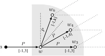
We can now unravelK0into a modelIofKby construct-ing a sequence of interpretationsIk = (∆Ik,·Ik), where Ik+1 extendsIk, and settingI = Sk≥0Ik. First we use

K0 to defineI0 by taking∆I0 = {a},AI0[−1,3] = {a},

AI0[i,j] _{=∅for all other intervals, andP}I0[i,j] _{=∅for all} [i, j]. We then observe that, inI0,ahas a ‘defect’ in the

a

w P

[-1,3]

w3

P

[-1,3]

w4

P _[-1,4]

wk

P [-1,k]

Figure 4: The unravelling construction.

interpretationI1by adding to∆I0 a (fresh) copywofdP

−

2

and settingPI1[−1,3] _{= {(a, w)} andP}I1[i,j] _{= ∅ for all}

other intervals. But now the newly introduced elementwin

I1has a defect in every interval[−1, k],k≥3, because it

does not have a requiredP-successor: indeed,dP−

2 belongs

to EP in every such interval in the canonical interpreta-tion of(T0_{, P(d}P

2, dP

−

2 ,−1,3)). To cure those defects, we

add toI1fresh copieswk ofdP −

2 , fork ≥3, and then set

PI2[−1,k] _{={(w, w}

k)}andPI2[i,j] =∅for all other

inter-vals, and so forth (see Fig. 4). The proof of Theorem 13 below shows thatI |=KiffK0 |=T0_.

Clearly, any KBKhas at least one witness ABox.

Theorem 13. Kis satisfiable iff there exists a witness ABox A0_{forKsuch thatK}0 _|=T0_.

The proof of (⇐), illustrated by Example 12, uses an unravelling technique similar to that of (Artale et al. 2014b, Theorem 4.1 and Lemma 6.5) developed for point-based temporalDL-Lite. An essential difference from the earlier construction is that now we not onlyshiftthe interpretation underlying the timeline of witnessesdR

δ in order to cure a

defect, but alsostretch(using Lemma 7) some intervals in these interpretations.

To show (⇒), we first construct aminimalwitness ABox

A0_{forKby taking(T}0_{,A)and recursively adding toAthe}

missing witnessesP(dP δ, d

P−

δ ,0, δ). In fact, we prove that

a fixed point in this construction will be reached in polyno-mially many steps. Then we consider the unravelling of the canonical interpretationK0forK0 _{= (T}0_,A0_{)and show that}

it is homomorphically embeddable into any model ofK. That

K0|=T0_{follows now by the construction of the unravelling.}

As a consequence of this proof we finally obtain:

Theorem 14. The satisfiability problem for HS-LiteH_horn[G]

KBs isP-complete.

Remark 15. Unfortunately, the construction above does not work for the wholeHS-LiteH_horn, where arbitrary operators

[R]can be used in the definition of temporal rolesS. To see why, consider first theHS-LiteH_horn[G] KBK = (T,A)with

T ={Av ∃P, P v[G]S}andA={A(a,0,0)}. Then aI∈(∃S)I[i,j]for anyI |=Kandi≤j. The axioms ofT2

make sure thataI∈ESI[i,j]_.

Consider now theHS-LiteH_horn KB K0 _{= (T}0_{,A) with}

T ={Av[G]∃P, P v[A]P1, P v[ ¯A]P2, P1uP2vS}.

We then haveaI ∈ (∃S)I[i,i], for anyI |=K0_{andi ∈}

Z.

However, it is not clear what axioms ofT2could make sure

thataI ∈ESI[i,i]_.

Data Complexity of Instance Checking

One of the main reasoning problems in description logic is

instance checking. In our context it can be formulated as follows: given a KB K = (T,A)and an atomC(a, i, j), whereCis a concept,aan individual name andi≤j, decide whetherK |=C(a, i, j). As instance checking is reducible to satisfiability, it is P-complete for bothHS-LiteHhorn/flatand HS-LiteH_horn[G]for combined complexity. Moreover, as a con-sequence of Theorems 10, 11 and 14, we also obtain:

Theorem 16. Instance checking for bothHS-LiteH_horn/flatand HS-LiteH_horn[G]isP-complete for data complexity(when only the ABox is regarded to be the input).

This result contrasts with the lower data complexity (AC0 and NC1) of instance checking with point-based temporal

DL-Lite(Artale et al. 2013; 2014a).

Outlook

Our interest in tractable description logics with interval-based temporal operators is motivated by possible applications in ontology-based data access (OBDA) over temporal databases. In the OBDA paradigm, one can query data sources,D, using the vocabulary of an ontology,T, that provides a unifying conceptual view of the data and enriches it with background knowledge (Calvanese et al. 2007). Given a query, q, an OBDA system rewritesqandT into another query,q0, such thatT, D |=qiffD|=q0, for any dataD. A standard on-tology language that guarantees the existence of a first-order rewritingq0_{is the OWL 2 QL profile of the Web Ontology}

Language OWL 2. (In a nutshell, OWL 2 QL isDL-LiteH_horn

in which concept and role inclusions cannot haveuon the left-hand side.) In the context oftemporal databases, we are interested in suitable ontology and query languages with temporal constructs (although some authors advocate the use of standard OWL 2 QL with temporal queries (Klarman 2014; Borgwardt, Lippmann, and Thost 2013)).

As modern temporal databases adopt the (downward hered-itary) interval-based model of time (Kulkarni and Michels 2012) and use coalescing to group time points into inter-vals (B¨ohlen, Snodgrass, and Soo 1996), in this paper we have launched an investigation of ontology languages that can be suitable for OBDA over such databases by design-ing the language HS-LiteH_horn and its tractable fragments

HS-LiteH_horn/flat and HS-LiteH_horn[G]. In view of Theorem 16, these languages cannot guarantee first-order rewritability of even atomic queries, though we believe datalog rewritings are possible. We leave the query rewritability issues, in par-ticular, the design ofDL-LiteHcore-based fragments supporting

References

Allen, J. 1981. An interval based representation of temporal knowl-edge. InProc. of the 7th Int. Joint Conf. on Artificial Intelligence (IJCAI-81), 221–226. Morgan Kaufmann.

Artale, A.; Kontchakov, R.; Lutz, C.; Wolter, F.; and Zakharyaschev, M. 2007. Temporalising tractable description logics. InProc. of the 14th Int. Symp. on Temporal Representation and Reasoning (TIME 2007), 11–22. IEEE Computer Society.

Artale, A.; Calvanese, D.; Kontchakov, R.; and Zakharyaschev, M. 2009. The DL-Lite family and relations.J. Artificial Intelligence Res. (JAIR)36:1–69.

Artale, A.; Kontchakov, R.; Wolter, F.; and Zakharyaschev, M. 2013. Temporal description logic for ontology-based data access. InProc. of the 23rd Int. Joint Conf. on Artificial Intelligence (IJCAI 2013), 711–717. IJCAI/AAAI.

Artale, A.; Kontchakov, R.; Kovtunova, A.; Ryzhikov, V.; Wolter, F.; and Zakharyaschev, M. 2014a. Temporal OBDA with LTL and DL-Lite. InProc. of the 2014 Int. Workshop on Description Logics

(DL 2014), 21–32. CEUR-WS.

Artale, A.; Kontchakov, R.; Ryzhikov, V.; and Zakharyaschev, M. 2014b. A cookbook for temporal conceptual data modelling with description logics.ACM Trans. Comput. Log.15(3):25.

Artale, A.; Kontchakov, R.; Ryzhikov, V.; and Zakharyaschev, M. 2015. Tractable interval temporal propositional and description logics. Full version available at www.dcs.bbk.ac.uk/∼_{roman/papers/}

aaai15-interval.pdf.

B¨ohlen, M. H.; Snodgrass, R. T.; and Soo, M. D. 1996. Coalescing in temporal databases. InProc. of the 22nd Int. Conf. on Very Large Data Bases (VLDB’96), 180–191. Morgan Kaufmann.

Borgwardt, S.; Lippmann, M.; and Thost, V. 2013. Temporal query answering in the description logic DL-Lite. InProc. of the 9th Int. Symp. on Frontiers of Combining Systems (FroCoS 2013), volume 8152 ofLNCS, 165–180. Springer.

Bresolin, D.; Goranko, V.; Montanari, A.; and Sciavicco, G. 2009. Propositional interval neighborhood logics: Expressiveness, de-cidability, and undecidable extensions. Ann. Pure Appl. Logic

161(3):289–304.

Bresolin, D.; Della Monica, D.; Montanari, A.; Sala, P.; and Sciav-icco, G. 2012a. Interval temporal logics over finite linear orders: the complete picture. InProc. of the 20th European Conf. on Artificial Intelligence (ECAI 2012), 199–204. IOS Press.

Bresolin, D.; Della Monica, D.; Montanari, A.; Sala, P.; and Sci-avicco, G. 2012b. Interval temporal logics over strongly discrete linear orders: the complete picture. InProc. of the 3rd Int. Symp. on Games, Automata, Logics and Formal Verification (GandALF 2012), volume 96 ofEPTCS, 155–168.

Bresolin, D.; Della Monica, D.; Goranko, V.; Montanari, A.; and Sci-avicco, G. 2014a. The dark side of interval temporal logic: marking the undecidability border.Ann. Math. Artif. Intell.71(1–3):41–83. Bresolin, D.; Della Monica, D.; Montanari, A.; and Sciavicco, G. 2014b. The light side of interval temporal logic: the Bernays-Sch¨onfinkel fragment of CDT. Ann. Math. Artif. Intell.

71(1–3):11–39.

Bresolin, D.; Mu˜noz-Velasco, E.; and Sciavicco, G. 2014. Sub-propositional fragments of the interval temporal logic of Allen’s relations. InProc. of the 14th European Conf. on Logics in Artificial Intelligence (JELIA’14), volume 8761 ofLNCS, 314–318. Springer. Calvanese, D.; De Giacomo, G.; Lembo, D.; Lenzerini, M.; and Rosati, R. 2007. Tractable reasoning and efficient query answer-ing in description logics: TheDL-Litefamily. J. Autom. Reason.

39(3):385–429.

Fisher, M.; Dixon, C.; and Peim, M. 2001. Clausal temporal resolution.ACM Trans. Comput. Log.2(1):12–56.

Gabelaia, D.; Kurucz, A.; Wolter, F.; and Zakharyaschev, M. 2005. Products of ‘transitive’ modal logics.J. Symb. Log.70(3):993–1021. Gabelaia, D.; Kurucz, A.; Wolter, F.; and Zakharyaschev, M. 2006. Non-primitive recursive decidability of products of modal logics with expanding domains.Ann. Pure Appl. Logic142(1–3):245–268. Greenlaw, R.; Hoover, H. J.; and Ruzzo, W. L. 1995. Limits to parallel computation: P-completeness theory. Oxford University Press.

Halpern, J. Y., and Shoham, Y. 1991. A propositional modal logic of time intervals.J. ACM38(4):935–962.

Hampson, C., and Kurucz, A. 2014. Undecidable propositional bimodal logics and one-variable first-order linear temporal logics with counting.CoRRabs/1407.1386.

Klarman, S. 2014. Practical querying of temporal data via OWL 2 QL and SQL:2011. In Short Papers Proc. of the 19th Int. Conf. on Logic for Programming, Artificial Intelligence and Reasoning (LPAR-19), volume 26 ofEPiC Series, 52–61. Easy-Chair.

Konev, B.; Wolter, F.; and Zakharyaschev, M. 2005. Temporal logics over transitive states. InProc. of the 20th Int. Conf. on Automated Deduction (CADE-20), volume 3632 ofLNCS, 182–203. Springer. Kulkarni, K. G., and Michels, J.-E. 2012. Temporal features in SQL:2011.SIGMOD Record41(3):34–43.

Lodaya, K. 2000. Sharpening the undecidability of interval temporal logic. InProc. of the 6th Asian Computing Science Conference (ASIAN 2000), volume 1961 ofLNCS, 290–298. Springer. Marcinkowski, J., and Michaliszyn, J. 2014. The undecidability of the logic of subintervals.Fundam. Inform.131(2):217–240. Marx, M., and Reynolds, M. 1999. Undecidability of compass logic.

J. Log. Comput.9(6):897–914.

Marx, M., and Venema, Y. 1997.Multi-dimensional Modal Logic, volume 4 ofApplied Logic. Kluwer Academic Publishers. Miyano, S.; Shiraishi, S.; and Shoudai, T. 1990. A list of P-complete problems. Technical Report RIFIS-TR-CS-17, Kyushu University. Montanari, A.; Puppis, G.; and Sala, P. 2014. Decidability of the interval temporal logicAAB¯ B¯over the rationals. InProc. of the 39th Int. Symp. on Mathematical Foundations of Computer Science (MFCS 2014), Part I, volume 8634 ofLNCS, 451–463. Springer. Reynolds, M., and Zakharyaschev, M. 2001. On the products of linear modal logics. J. Log. Comput.11(6):909–931.