Bonner, Stephen Arthur Robert
Using Hadoop to implement a semantic method for assessing the quality of medical data
Original Citation
Bonner, Stephen Arthur Robert (2014) Using Hadoop to implement a semantic method for assessing
the quality of medical data. Masters thesis, University of Huddersfield.
This version is available at http://eprints.hud.ac.uk/id/eprint/23305/
The University Repository is a digital collection of the research output of the
University, available on Open Access. Copyright and Moral Rights for the items
on this site are retained by the individual author and/or other copyright owners.
Users may access full items free of charge; copies of full text items generally
can be reproduced, displayed or performed and given to third parties in any
format or medium for personal research or study, educational or notforprofit
purposes without prior permission or charge, provided:
•
The authors, title and full bibliographic details is credited in any copy;
•
A hyperlink and/or URL is included for the original metadata page; and
•
The content is not changed in any way.
For more information, including our policy and submission procedure, please
contact the Repository Team at: [email protected].
Using Hadoop To Implement A Semantic
Method For Assessing The Quality Of
Medical Data
Author:
Stephen BONNER
Supervisor:
Prof. Grigoris ANTONIOU
A thesis submitted to the University of Huddersfield
in partial fulfilment of the requirements for the degree of Masters By Research
High Performance Computing School Of Computing and Engineering
Copyright Statement
i. The author of this thesis (including any appendices and/or schedules to this thesis) owns any copyright in it (the “Copyright”) and s/he has given The University of Huddersfield the right to use such Copyright for any administrative, promotional, educational and/or teaching purposes.
ii. Copies of this thesis, either in full or in extracts, may be made only in accordance with the regulations of the University Library. Details of these regulations may be obtained from the Librarian. This page must form part of any such copies made.
opinions drown out your own inner voice. And most important, have the courage to follow
your heart and intuition.”
Steve Jobs 2005
“The secret of the mountain is that the mountains simply exist, as I do myself: the
moun-tains exist simply, which I do not. The mounmoun-tains have no ”meaning,” they are meaning; the
mountains are. I understand all this, not in my mind but in my heart, knowing how
meaning-less it is to try to capture what cannot be expressed, knowing that mere words will remain
when I read it all again, another day.”
Peter Matthiessen 1978
“If you don’t know, the thing to do is not to get scared, but to learn.”
Recent technological advances in modern healthcare have lead to a vast wealth of patient data being collected. This data is not only utilised for diagnosis but also has the potential to be used for medical research. However, there are often many errors in datasets used for medical research, with one study finding error rates ranging from 2.3% to 26.9% in a selection of medical research databases.
I would like to thank the many people who have supported and helped me with this thesis. I would firstly like to thank my parents, Dr Louise Bonner and Mr Neil Bonner, for all their incredible and unwavering support during my academic career. I would also like to thank my supervisory team of Professor Grigoris Antoniou and Dr Violeta Holmes. I would also like to thank Dr Laura Moss and Dr David Corsar for their original effort in this work and for allowing me to expand upon it.
I would like to thank all of my family and friends, of which there are too many to mention in full here, but I would like to mention Holly Lewis, Joseph Luke, Olive Chittock, Liam lane, Professor Fiona Tweed, Dave Guldin, Barbara Hughes, Dr John Ambrose and Neil MacGregor.
I would like to thank all my friends and colleges at the University Of Huddersfield and specif-ically the members of the High Performance Computing Research Group: Ibad Kureshi, John Brennan, Mathew Newall, Shuo Liang and Yvonne James. I would also like to ac-knowledge the open-source software community, particularly: Apache (For their continued work on Hadoop) and the Linux Foundation. I would also like to acknowledge the use of the University of Huddersfield Queensgate Grid in carrying out this work.
Abstract 3
Acknowledgements 4
Contents 5
List of Figures 11
List of Tables 14
List of Algorithms 15
Abbreviations 16
1 Introduction 17
1.1 Errors In Medical Databases . . . 17
1.2 Current Possible Solutions Using Linked Open Data . . . 18
1.2.1 The Semantic Web and Linked Open Data . . . 18
1.2.2 Big Data and Healthcare . . . 19
1.2.3 Current Implementation . . . 20
1.3 Project Aims and Motivations . . . 21
2 Background Technologies 22 2.1 The Resource Description Framework (RDF) . . . 22
2.1.1 An RDF Statement . . . 23
2.1.2 RDF Graph Representation . . . 23
2.1.3 RDF Serialisation Formats . . . 24
2.2 Triplestores . . . 26
2.2.1 Jena . . . 26
2.3 Simple Protocol and RDF Query Language (SPARQL) . . . 27
2.4 Database Joins . . . 28
2.5 Hadoop And The Map/Reduce Programming Model . . . 29
2.5.1 Hadoop Cluster Components . . . 30
2.5.2 The Hadoop Distributed File System (HDFS) . . . 30
2.5.3 Map/Reduce Programming Model . . . 31
2.5.4 Sort/Shuffle, Partitioner and Combiner Stages . . . 32
2.5.5 Benefits and Drawbacks . . . 33
2.5.6 Associated Technologies . . . 34
3 Literature Review 36 3.1 Research Fields . . . 36
3.2 Distributed Native Triplestores . . . 37
3.3 Performing Dataset Joins Via Hadoop . . . 38
3.3.1 Map-Side Join . . . 39
3.3.2 Reduce-Side Join . . . 40
3.3.3 Cascade Join . . . 41
3.3.4 Broadcast Join . . . 42
3.4 Feasibility Of Using Hadoop For RDF Processing . . . 42
3.5 Strategies For Storing RDF Data On The HDFS . . . 43
3.6 Queries on RDF Data Using Map/Reduce . . . 44
3.6.1 Existing Theoretical Approaches . . . 44
3.6.2 Presented Performance Results . . . 51
3.7 Limitations Of Existing Hadoop RDF Solutions . . . 53
3.7.1 Hadoop Joining Strategies . . . 54
3.7.2 Data Upload Stages . . . 55
4 Analysis Of Current Jena TDB Implementation 57
4.1 Current Implementation . . . 57
4.2 Limitations of Existing Solution . . . 58
4.3 Current Implementation Performance Analysis . . . 59
4.3.1 Upload Time . . . 59
4.3.2 Query Time . . . 59
4.3.3 Analysis . . . 60
4.4 The Need For A New Framework . . . 61
5 Hadoop Implementation and Algorithm Design 62 5.1 Structure and Distribution Of The Real-World Medical Data . . . 62
5.1.1 Subject, Predicate and Object Distribution . . . 63
5.1.2 Distinct Triple Group Distribution . . . 63
5.2 Data Generation . . . 64
5.3 Analysis Of Current SPARQL Queries . . . 64
5.3.1 Min/Max Queries . . . 65
5.3.2 More Complex Queries . . . 66
5.4 Hadoop-Based Framework Design . . . 67
5.4.1 Required Software Functionality . . . 67
5.4.2 Why Use Hadoop As The Basis For The New Framework? . . . 68
5.4.3 The Two Approaches Taken . . . 68
5.5 Query Planning . . . 69
5.6 Approach One - Data Upload Algorithm . . . 70
5.6.1 Stage One - Compression . . . 72
5.6.2 Stage Two - Sort On Subject . . . 72
5.6.3 Algorithm Pseudocode . . . 73
5.7 Approach One - Data Query Algorithm Design and Joining Strategies . . . . 73
5.7.1 Selection Stage . . . 75
5.7.2 Join Stage . . . 78
5.8 Approach Two . . . 81
5.8.2 Join Phase . . . 82
5.9 Implementation Summary . . . 83
5.9.1 Key Theoretical Performance Advantages . . . 83
5.9.2 Summary . . . 83
6 Test Environment and Optimisations 86 6.1 Details Of Test Environments . . . 86
6.1.1 Single Machine . . . 86
6.1.2 Dedicated Hadoop Cluster . . . 87
6.2 Hadoop Cluster Performance Optimisations . . . 87
6.2.1 Benchmark Generation . . . 88
6.2.2 Optimum Number Of Map/Reduce Tasks . . . 88
6.2.3 Optimum JVM Heap Memory Allocation . . . 89
6.2.4 JVM Re-use . . . 91
6.2.5 Sort Memory Allocation . . . 92
6.2.6 Final Configuration Values . . . 92
7 Results 94 7.1 Testing Methodology . . . 94
7.2 Single Node Results . . . 95
7.3 Single Node Results - Approach One . . . 95
7.3.1 Upload Results . . . 95
7.3.2 Upload Results Showing Breakdown Of Passes . . . 95
7.3.3 Query Results . . . 97
7.3.4 Query Results Showing Breakdown Of Passes . . . 97
7.4 Single Node Results - Approach Two . . . 98
7.4.1 Query Results . . . 98
7.4.2 Query Results Showing Breakdown Of Passes . . . 99
7.5 Single Node Comparison . . . 99
7.5.1 Approach Comparison . . . 99
7.6 Hadoop Cluster Results . . . 103
7.7 Cluster Results - Approach One . . . 103
7.7.1 Upload Performance Across Eight Nodes . . . 103
7.7.2 Query Performance Across Eight Nodes . . . 104
7.7.3 Performance Scalability Across Number Of Nodes . . . 104
7.7.4 Speed-Up Analysis Of Approach One’s Query Stage . . . 105
7.8 Cluster Results - Approach Two . . . 106
7.8.1 Query Performance Across Eight Nodes . . . 106
7.8.2 Performance Scalability Across Number Of Nodes . . . 108
7.8.3 Speed-Up Analysis Of Approach Two’s Query Stage . . . 108
7.9 Cluster Approach Comparison . . . 109
7.9.1 Approach Comparison On Eight Nodes . . . 109
7.9.2 Approach Comparison On Four Nodes . . . 111
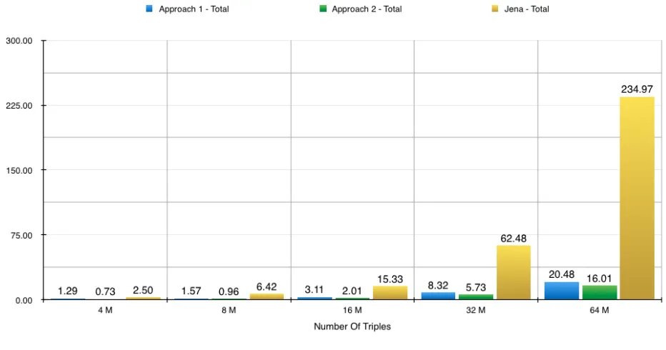
7.9.3 Approach Comparison With Jena . . . 111
7.10 Na¨ıve versus Optimised Implementation . . . 112
8 Interpretation and Discussion Of Results 114 8.1 Summary and Significance Of Results . . . 114
8.1.1 Single Node Results . . . 114
8.1.2 Cluster Results . . . 115
8.1.3 Cluster Size Versus Speed-Up Factor . . . 115
8.1.4 Approach Comparison . . . 116
8.1.5 Underlying Pass Comparison . . . 118
8.2 Comparison With Literature . . . 118
9 Conclusions And Further Work 121 9.1 Conclusions . . . 121
9.1.1 Project Summary . . . 121
9.1.2 Aims and Objectives Achieved . . . 122
9.1.3 Evaluative Conclusions . . . 122
9.2.1 Improvements To The Project . . . 124
9.2.2 Expansion Of The Project . . . 125
9.3 Final Conclusions . . . 126
References 128 A Appendix - SPARQL Queries 134 A.1 Original SPARQL Queries . . . 134
B Appendix - Hadoop Cluster Configuration Files 138 B.1 HDFS Site . . . 138
B.2 Mapred Site . . . 138
B.3 Core Site . . . 139
C Appendix - Approach One Source Code 140 C.1 Upload Algorithm . . . 140
C.1.1 Map 1 - Compressor . . . 140
C.1.2 Map 2 - Create Single Line On Subject . . . 142
C.1.3 Reduce 1 - Create Single Line On Subject . . . 143
C.2 Query Algorithm . . . 143
C.2.1 Map 1 - Pass 1 . . . 143
C.2.2 Reduce 1 - Pass 1 . . . 146
C.2.3 Map 2 - Pass 2 . . . 149
C.2.4 Reduce 2 - Pass 2 . . . 150
D Appendix - Approach Two Source Code 158 D.1 Query Algorithm . . . 158
D.1.1 Map 1 - Pass 1 . . . 158
D.1.2 Reduce 1 - Pass 1 . . . 161
D.1.3 Map 2 - Pass 2 . . . 165
D.1.4 Reduce 2 - Pass 2 . . . 165
1.1 The Semantic Web Stack . . . 18
1.2 Real World Open Linked Data . . . 19
2.1 A Sample RDF Dataset . . . 24
2.2 Graphic Representation Of RDF Data . . . 24
2.3 Basic Map/Reduce Workflow . . . 31
2.4 Full Map/Reduce Workflow . . . 33
3.1 SPARQL Map/Reduce Research Areas . . . 36
3.2 Map-Side Join . . . 39
3.3 Reduce-Side Join . . . 40
3.4 Kulkarni’s Selection Phase . . . 46
3.5 Kulkarni’s Join Phase . . . 47
3.6 Mazumdar’s Example SPARQL Query . . . 47
3.7 Mazumdar’s Query Execution Plan . . . 48
3.8 Mazumdar’s First Join . . . 48
3.9 Goasdoue’s 1-Clique Query . . . 50
3.10 Goasdoue’s Central Clique Query . . . 50
3.11 Mazumdar’s Performance Results . . . 51
3.12 Husain’s Performance Results . . . 52
3.13 Goasdoue’s Upload Performance Results . . . 53
3.14 Goasdoue’s Query Performance Results . . . 53
4.1 Current Approach For Checking Medical Data . . . 58
4.3 Jena TDB Query Performance . . . 60
5.1 Triple Group Joining Plan . . . 71
5.2 Approach One - Selection Stage Workflow . . . 75
5.3 Map-Side Join Example . . . 76
5.4 Reduce-Side Join Example . . . 77
5.5 Join Stage Workflow . . . 79
5.6 Hadoop Job Output Showing Counters . . . 81
5.7 Approach Two - Selection Stage Workflow . . . 82
6.1 Number of Map/Reduce Tasks Results . . . 89
6.2 Hadoop Memory Footprint Calculation . . . 90
6.3 Optimum Heap Size Result . . . 90
6.4 JVM Reuse Result . . . 91
6.5 Hadoop Sort IO Result . . . 92
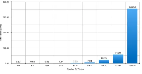
7.1 Approach One - Single Machine Upload Time . . . 96
7.2 Approach One - Single Machine Upload Time Showing Breakdown Of Passes 96 7.3 Approach One - Single Machine Query Time . . . 97
7.4 Approach One - Single Machine Query Time Showing Selection And Join Stages . . . 98
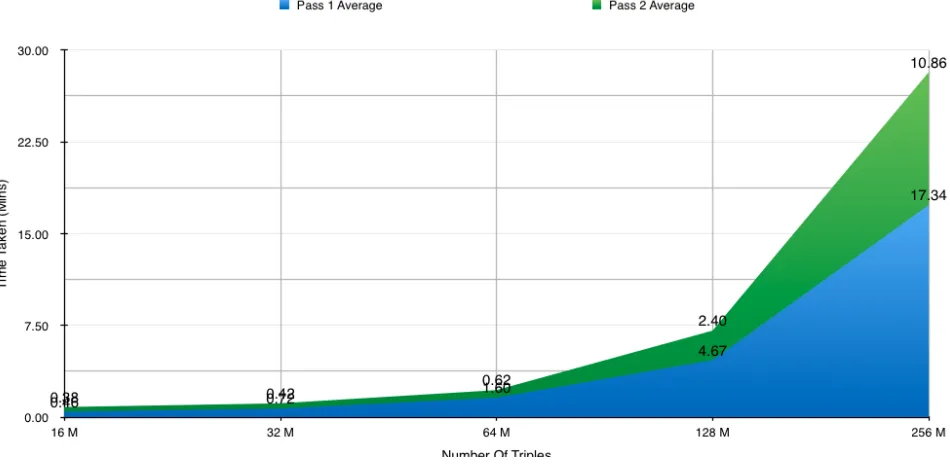
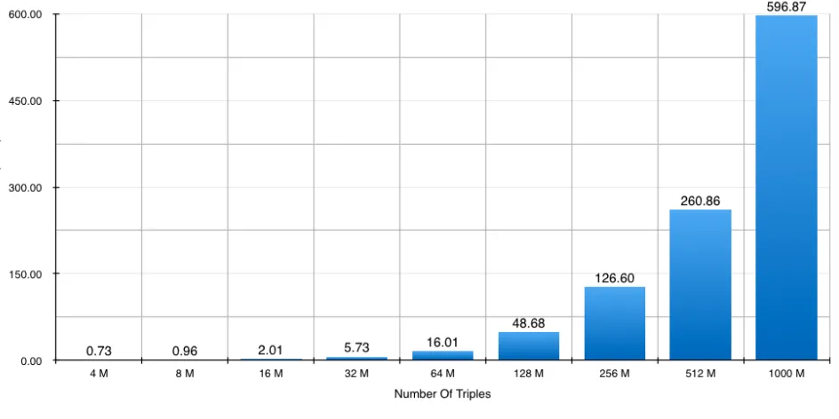
7.5 Approach Two - Single Machine Query Time . . . 99
7.6 Approach Two - Single Machine Query Time Showing Pass Breakdown . . . 100
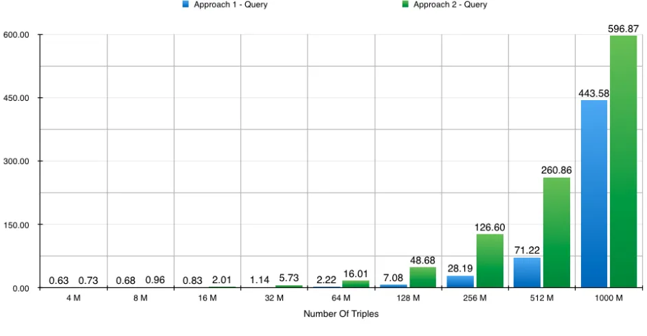
7.7 Single Node Query Performance Comparison Between Approaches . . . 101
7.8 Single Node Total Performance Comparison Between Approaches . . . 101
7.9 Single Node Total Performance Comparison Between Hadoop And Jena . . . 102
7.10 Approach One - Upload Performance Across 8 Nodes . . . 103
7.11 Approach One - Query Performance Across 8 Nodes . . . 104
7.12 Approach One - Upload Performance Scalability Across Nodes . . . 105
7.13 Approach One - Query Performance Scalability Across Nodes . . . 106
7.14 Approach One - Query Speed-Up Factor . . . 107
7.16 Approach Two - Query Performance Scalability Across Nodes . . . 108
7.17 Approach Two - Query speed-up Factor . . . 109
7.18 Eight Node Cluster Approach Query Comparison . . . 110
7.19 Eight Node Cluster Approach Total Comparison . . . 110
7.20 Four Node Cluster Approach Total Comparison . . . 111
7.21 Hadoop Approaches Versus Jena . . . 112
2.1 Join Example 1 . . . 29
2.2 Join Example 2 . . . 29
2.3 Join of Table 1 and 2 on Course-ID . . . 29
5.1 Subject, Predicate and Object Distribution . . . 63
5.2 Triple Group Distribution . . . 63
6.1 Specification Of The Single Machine . . . 86
6.2 Specification Of The Hadoop Cluster . . . 87
6.3 Hadoop Configuration Files . . . 88
6.4 Hadoop Memory Allocation on Cluster . . . 91
6.5 Hadoop Cluster Final Configuration Values . . . 93
8.1 Specification Of The Clique-Square Hadoop Cluster . . . 119
1 Medical Data Upload Algorithm . . . 74 2 Medical Data Query Map/Reduce Iteration 1 . . . 78 3 Medical Data Query Map/Reduce Iteration 2 . . . 85
RDF ResourceDescriptionFramework
SPARQL SimpleProtocolAndRDFQueryLanguage
URI UniformResourceIdentifiers
URL UniformResourceLocator
HDFS HadoopDistributedFileSystem
JVM JavaVirtualMachine
RAM RandomAccessMemory
BGP BasicGraphPatern
NHS NationalHealthService
LUBM LehighUniversityBenchmark
Introduction
1.1
Errors In Medical Databases
Recent technological advances in modern healthcare have led to a vast wealth of patient data being collected. This data is not only utilised for diagnosis but also has the potential to be used for medical research. For any conclusions from this research to be of worth, the underlying data needs to be of high quality. However, according to Goldberg, Niemierko, and Turchin (2008), there are often many errors in datasets used for medical research. In this study they found error rates ranging from 2.3% to 26.9% in a selection of medical research databases. Salati et al. (2011) highlight a series of metrics on which the quality of medical data can be judged. These are accuracy, completeness, consistency and believability. Salati et al. (2011) state that the errors which they find present in medical databases can have three different etiologies: firstly, errors which were present in the original data and then copied into the medical databases; secondly, errors which occur due to misinterpretation of the original data; finally, errors which occur when the data is being entered into the database. With such high error rates present in medical databases there is clear need for a system to assess the quality of data before it is used as the basis of cutting edge research.
1.2
Current Possible Solutions Using Linked Open Data
There has been an attempt to create a system which automatically assesses a given dataset to check for errors contained within (Corsar, Moss, & Piper, 2012). Such a system has been developed using Semantic Web and Linked Open Data technologies, both of which will be expanded upon in this section. The concepts relating to the emerging field of Big Data and how this relates to healthcare will also be explored.
1.2.1 The Semantic Web and Linked Open Data
The original vision of the Semantic Web was established by Berners-Lee, Hendler, and Lassila (2001). The vision was to create a machine-readable structure to supplement the pre-existing human-readable content of web pages. According to Davies, Fensel, and van Harmelen (2003) this structure consists of meta-information, defining specific properties about any given element of data. This meta-information captures some of the meaning, or semantics behind the data, leading to the concept being named the Semantic Web (Antoniou & Harmelen, 2008). The Semantic Web is implemented in a series of layers, which collectively form the Semantic Web stack illustrated in Figure 1.1. A more in-depth view of one of the fundamental layers of the Semantic Web, the Resource Description Framework (RDF), can be found in Chapter 2.
Linked Open Data is defined by Bizer, Heath, and Berners-Lee (2009) as being simply different sources of data which are inter-linked together via the web. These data sources can be geographically distributed and vary in source, content and format. To enable these datasets to be linked, Semantic Web technologies and concepts are utilised. The number of real-world datasets linked to others via the Open Linked Data philosophy is increasing rapidly as Figure 1.2 demonstrates.
FIGURE1.2: Real World Open Linked Datasets (Bizer et al., 2009).
1.2.2 Big Data and Healthcare
(2011), have not yet been fully realised. This is due to the technical challenges which stor-ing and processstor-ing the massive volume of data present. Gartner (2011) argues that it is not only the volume of data which is challenging current technology, but also the variety (the heterogeneity of data, representation, and semantic interpretation) and velocity (data arrival and required processing rate) of the data.
The biomedical and general healthcare fields have the potential to be one of the biggest con-tributors to and benefactors from the big data phenomenon. Feldman, Martin, and Skotnes (2012) state that the volume of worldwide healthcare data as of 2012 is estimated to be over 500 petabytes. This Figure is predicted to increase by a factor of 50 to a value of 25,000 petabytes by 2020. Agrawal et al. (2011) state that one of the biggest contributors to this data explosion will be the use of continuous monitoring machines, both in hospitals and at home. Howe et al. (2008) explain that analysing this data has the potential to alter biomedical research and significantly improve healthcare diagnosis.
1.2.3 Current Implementation
1.3
Project Aims and Motivations
Due to the potential volume of RDF-based medical records, performance issues with the current framework could limit its adoption in the wider medical community. This project will explore alternative methods for both storing medical RDF data and also assessing its quality via a series of SPARQL queries. One of the key considerations for this project will be performance and scalability of data upload and also query response time.
The specific aims and objectives of this project are as follows:
i ) To create a new storage and query framework for medical data, with specific emphasis being placed on performance. This will be implemented in Apache Hadoop Map/Reduce.
ii ) To test the newly developed Hadoop framework using real-world medical data.
Background Technologies
In this chapter the fundamental, underlying technologies utilised in this project will be intro-duced and explained. These technologies include RDF, SPARQL, Triplestores, Hadoop and the Map/Reduce programming model.
2.1
The Resource Description Framework (RDF)
The Resource Description Framework (RDF) is one of the fundamental layers of the se-mantic web stack illustrated in Figure 1.1. According to W3C (2004) RDF is a language specifically designed to express the relationship between elements on the world wide web. The philosophy behind RDF is about making statements that are easy for machines or com-puter programs to understand and process.
Antoniou and Harmelen (2008) state that the fundamental concepts of RDF can be consid-ered to be: Resources, Properties and Statements.
• Resources are objects or things, about which there is a need to express some infor-mation. Resources are represented by Uniform Resource Identifiers (URI) which is a unique way of identifying a specific Resource.
• Properties describe the relationship between different Resources. Each Property is also identified via a URI.
• Statements are the complete RDF triple. An RDF triple consists of a Resource, a Property and a Value. Values can be a Resource or literals (such as a string or inte-ger).
2.1.1 An RDF Statement
Ogbuji (2000) states that an RDF Statement comprises three distinct structural components: a Subject (about which the statement is being made), a Predicate (describing the relation-ship between Subject and Object) and an Object (an attribute of the Subject). Ogbuji (2000) expands upon the concept of an RDF Statement by drawing comparisons with the English language. For example the sentence’John Brennan is a lecturer at the University of Hud-dersfield’ can be represented in RDF with the following structure:
• Subject (’John Brennan’)
• Predicate (’lecturer at’)
• Object (’University of Huddersfield’)
Resources in RDF, as previously discussed, are represented by URI’s. A Uniform Resource Locator (URL) is a subset of URI’s which is often used to locate an RDF Resource. There-fore the statement from earlier could more accurately be represented as:
• Subject (http://www.hud.ac.uk/staff/John Brennan)
• Predicate (http://www.hud.ac.uk/role/lecturer)
• Object (http://www.hud.ac.uk)
2.1.2 RDF Graph Representation
useful in visualising how simple RDF triple statements can be built up to express complex relationships between numerous unique resources.
FIGURE2.1: A Sample RDF Dataset (Goasdou ´e et al., 2013).
FIGURE2.2: Graphic Representation Of Sample RDF Data (Goasdou ´e et al., 2013).
2.1.3 RDF Serialisation Formats
Segaran, Evans, and Taylor (2009) explain that there are several formats in which an RDF statement can be serialised, including RDF/XML, N3 and N-Triple. The original RDF seri-alisation is RDF/XML, which builds on the XML structure of tags to represent a Triple. The earlier statement would be expressed in RDF/XML as:
<?xml version="1.0" encoding="UTF-16"?> <rdf:RDF
xmlns:rdf="http://www.w3.org/1999/02/22-rdf-syntax-ns" xmlns:unidomain="http://www.hud.ac.uk/my-rdf-ns">
</rdf:Description> </rdf:RDF>
The N-Triple notation is a simpler way of representing an RDF Triple. Each line of N-Triple contains a single RDF Statement in full, with the subject, predicate and object separated by whitespace. Both Subject and Object are represented as a full URI enclosed by angle brackets. The earlier statement would be expressed in N-Triple as:
<http://www.hud.ac.uk/staff/John_Brennan>
<http://www.hud.ac.uk/role-/lecturer> <http://www.hud.ac.uk>
While the structure of N-Triple is extremely simple, it can lead to a lot of repetition with larger RDF datasets. It is common for RDF datasets to contain numerous statements that share at least one element, which the N-Triple format will repeat. The N-Triple format also expresses RDF data with the full URI, again a wasteful method.
The N3 format attempts to rectify some of the inherent inefficiencies with the N-Triple for-mat. It does this via two methods. Firstly, N3 replicates the XML namespace mechanism to allow definition of URI prefixes at the beginning of a RDF document. Secondly, N3 pro-vides a method of representing statements that share a common element. For example the statement from earlier could be expanded on in N3 as:
@prefix rdf: <http://www.w3.org/1999/02/22-rdf-syntax-ns#>.
@prefix foaf: <http://xmlns.com/foaf/0.1/>.
@prefix hud: <http://www.hud.ac.uk/#>.
hud:John_Brennan rdf:type foaf:person;
hud:lecture hud:uni.
2.2
Triplestores
A triplestore is a framework designed especially to provide persistent storage of and the ability to query RDF data Haslhofer, Roochi, Schandl, and Zander (2011). According to Sequenda (2013), triplestores can be categorised into three groups based on the storage implementation. These groups are Native, RDBMS-backed and NoSQL. Native triplestores are designed specifically for, and thus optimised for, storing RDF data. These Native imple-mentations are independent of other Relational Database Management Systems (RDBMS) and store the RDF data in the local filesystem. RDBMS-backed triplestores store the RDF data in a traditional relational database such as MySQL. NoSQL triplestores are a recent development designed to exploit the advances being made in NoSQL databases such as Cassandra.
According to Weaver and Williams (2009) while many of the common native triplestores use advanced database techniques to enable fast querying of RDF data, they require a lot of pre-processing which can often lead to a prohibitively long data upload time.
2.2.1 Jena
Jena is one of the mostly widely utilised tools used to store and process RDF data and was originally developed by Hewlett-Packard(Wilkinson, Sayers, Kuno, & Reynolds, 2003). It comprises a Java API, allowing users to write programs that create or manipulate RDF data, as well as a native (Jena TDB) and also a RDBMS-backed (Jena SDB) triplestore to house and query RDF data. Jena implements a query engine called ARQ to perform SPARQL queries on the triplestore.
2.3
Simple Protocol and RDF Query Language (SPARQL)
According to DuCharme (2011) the Simple Protocol and RDF Query Language (SPARQL) provides a way of querying RDF data stored in a triplestore and is the W3C standard for doing so. SPARQL can be compared to the Structured Query Language (SQL), used to query standard relational databases, as they share a similar syntax and logic. Antoniou and Harmelen (2008) expand on SPARQL by explaining that conceptually, it is based around matching graph patterns. According to W3C (2013), a query evaluates what is known as a basic graph pattern (BGP). Each BGP can contain several query patterns all resembling an RDF triple. Variables are able to substitute any part of the BGP to allow individual elements to be extracted from any input triples matching the rest of the pattern (W3C, 2013). Goasdou ´e et al. (2013) state that the normative syntax for a SPARQL query is:
SELECT ?v1...?vn WHERE {t1...tn}
with the SELECT ?v1...?vn element representing distinct variables occurring in the input data and the order in which they are to be returned. FROM is an optional element not shown, that can be utilised to determine the data source to be queried. The WHEREt1...tn element forms the BGP and is a series of triple query patterns that will match the graph of any input triples against the ones specified in the BGP.
A basic SPARQL query that selects all lecturers at the University of Huddersfield would be:
PREFIX rdf: <http://www.w3.org/1999/02/22-rdf-syntax-ns#> PREFIX hud: <http://www.hud.ac.uk/#> .
SELECT ?name WHERE
{
?name hud:Lecturer hud:Uni . }
PREFIX rdf: <http://www.w3.org/1999/02/22-rdf-syntax-ns#> PREFIX hud: <http://www.hud.ac.uk/#> .
SELECT ?name WHERE
{
?name hud:Lecturer hud:Uni . ?name hud:School hud:Computing . }
In this example the BGP has two query patterns to match, both of which share a common variable. According to DuCharme (2011), replicating a variable between two triple patterns in a SPARQL query is done to join together the two patterns. When the SPARQL query engine finds a triple with the predicate of hud:Lecturer and an object of hud:Uni it would bind the subject of such a triple to the variable ?name. When processing the second pat-tern, possible matches will be limited to results containing the variable ?name. Effectively results from the first pattern will be joined to results from the second so that only elements meeting both conditions will be returned. The process of joining data comes from the world of relational databases and is explored in the next section.
2.4
Database Joins
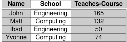
Table 2.1 and Table 2.2 contain data that will be joined via a natural join. In this example the values of the Teaches-Course from table 2.1 will be joined to 2.2 via the values from the Course-ID.
Name School Teaches-Course
John Engineering 165
Matt Computing 132
Ibad Engineering 50
Yvonne Computing 74
TABLE2.1: Join Example 1
Course-ID Course-Name
165 DSP
50 PCA
74 CS
TABLE2.2: Join Example 2
The join can be expressed as the following: (T eachesCourse ./ CourseID) → N ewT able
Joining the two datasets will create a new dataset shown in Table 2.3. All results that can join via the foreign key will be included in the table, while results not matching (for example the record for ’Matt’) will be absent.
Name School Teaches-Course Course-Name
John Engineering 165 DSP
Ibad Engineering 50 PCA
Yvonne Computing 74 CS
TABLE2.3: Join of Table 1 and 2 on Course-ID
2.5
Hadoop And The Map/Reduce Programming Model
[image:31.596.194.415.148.221.2] [image:31.596.154.458.448.510.2]2.5.1 Hadoop Cluster Components
According to Chandar (2010) a Hadoop cluster consists of the following components, all of which are Java Virtual Machines (JVM):
• JobTracker - Master node which controls the submission and scheduling of jobs on the cluster.
• NameNode- Controller node for the HDFS, which keeps track of which node stores what data.
• TaskTracker - These nodes are worker nodes for Map/Reduce and are where the processing happens. A TaskTracker demon does not itself run jobs, instead it controls the spawning of separate JVMs for each Map/Reduce function.
• DataNode- These nodes comprise the rest of the HDFS and house the data. Usually DataNodes are also TaskTrackers, so data can be processed on the same node in which the data resides.
2.5.2 The Hadoop Distributed File System (HDFS)
2.5.3 Map/Reduce Programming Model
Hadoop’s Java implementation of the Map/Reduce programming model is based on Google’s proprietary system introduced in a 2004 paper (Lam, 2010). According to Dean and Ghe-mawat (2004) a standard Map/Reduce pass consists of two distinct phases: a Mapper and a Reducer. All inputs to a Map/Reduce task are key/value pairs, with all intermediate and final output also represented in this way.
Dean and Ghemawat (2004) explain the role of each phase in the following manner: the Map function processes the input key/value pairs, performs a user-defined algorithm, then outputs an intermediate set of key/value pairs. These intermediate results are grouped on the key to ensure that all values associated with that key are sent to the same Reduce func-tion. The Reduce function then performs the final processing and outputs the last set of key/value pairs. The basic workflow of Map/Reduce is demonstrated in Figure 2.3.
FIGURE2.3: Simplified Map Reduce Workflow (Rajaraman & Ullman, 2012).
Reduce function would be (w1, [1 1 1 1 1]), for a word that had five instances in the original input files. The Reduce function then would sum the values for the key and emit the total, along with the word as the final output - (w1, 5).
The pseudocode for the word-count program would be:
Map:
void Map(string document) {
for each word w in document { Emit_Intermediate(w, "1");
Reduce:
void Reduce (string word, list<string> values) { int count = 0;
for each v in values { count += StringToInt(v); Emit_Final(word, count);
2.5.4 Sort/Shuffle, Partitioner and Combiner Stages
guarantee of access to all values for a specific key so they are only really utilised to reduce the amount of data to be passed to the final Reducer (Lin & Dyer, 2010).
The location of these additional stages in the Map/Reduce workflow can be seen in Figure 2.4.
FIGURE2.4: The Full Map Reduce Workflow (Lin & Dyer, 2010).
2.5.5 Benefits and Drawbacks
the network bottleneck can seriously limit the performance of the system. One of the major advantages of the Hadoop framework is that it tries to ensure that the data to be processed is available on the local drive of the compute node. This bypasses the need for a time-consuming network transfer of the data. This key feature, known as data locality, is one of the main drivers of Hadoop’s performance advantage (White, 2010).
Hadoop imposes strict limits on both the Map and Reduce functions to enable it to perform the parallelisation. Map functions inherently have to work independently on one set of key/-value pairs and have no access to other pairs. The Reduce function can only access those values associated with the key used to generate the reduce function, making features such as dataset joins complicated (White, 2010). Hadoop is implemented in Java, with each of the cluster components discussed in section 2.5.1 running as a separate JVM. During a standard Map/Reduce iteration each Map and Reduce task incurs a start-up penalty asso-ciated with spawning the JVM. Due to this penalty it is usually best to limit the number of passes required to complete a set task (Joshi, 2012). Another disadvantage that is asso-ciated with Hadoop is the steep learning curve in discovering how to correctly program a Map/Reduce job. White (2010) argues that creating a new Map/Reduce task even for an experienced programer is not a quick process due the complexity of the code and number of required functions for even a simple job.
2.5.6 Associated Technologies
There are a selection of other technologies under the Apache Hadoop banner which build extra functionality onto both the HDFS and Map/Reduce layers. These technologies include: H-Base, Hive and Pig.
Hive is a project created by Facebook to provide not only a structured data store, but also a way of querying the data via an SQL-like language called Hive QL (White, 2010). According to Taylor (2010) a query created using Hive QL is automatically translated into the required number of Map/Reduce tasks, enabling users who are familiar with SQL to easily start processing data via Hadoop. Hive will automatically perform any requested joins between data elements. However White (2010) shows that if multiple joins are required across data elements residing in different columns, Hive will perform an un-optimised and slow series of cascade joins (Cascade joins will be discussed further in section 3.3.3).
Literature Review
3.1
Research Fields
An analysis of literature from several different fields is required in order to successfully and efficiently devise a method to perform SPARQL queries via Map/Reduce. Figure 3.1 effectively demonstrates the overlap between the different fields from which this project draws. This chapter will explore prior research conducted into area 2 highlighted in Figure 3.1: performing SPARQL queries using Map/Reduce.
FIGURE3.1: SPARQL Map/Reduce Research Areas (Myung, 2010).
3.2
Distributed Native Triplestores
According to Owens, Seaborne, and Gibbins (2008) the volume of structured RDF data is quickly outstripping the ability of native triplestores to store and query. Many of the most commonly used triplestores are designed to only utilise a single machine. However, in an effort to improve both upload and query performance, there have been attempts to create distributed native triplestores that either augment or replace existing solutions.
Weaver and Williams (2009) developed a system that is able to process and query RDF data on a selection of HPC machines, ranging from commodity Beowulf clusters to IBM Blue Gene machines. Their implementation is created using the Message Passing Interface (MPI) to enable parallelisation and requires no processing of the data to be performed before it is stored. Weaver and Williams (2009) state that while their system performs well when compared with traditional triplestores, it requires that the entire RDF data set, along with all intermediate results, fit in the main system memory. They highlight that this approach has two clear disadvantages. Firstly, any machine must have an equal or greater amount of RAM to the size of the RDF dataset. This requirement would place a finite limit on dataset size as it could never exceed the size of system memory. Secondly, as RAM is volatile storage, this would not be an ideal solution to permanently house the data, as a hardware or power failure would result in complete data loss.
of three machines. On one such query, a Clustered TDB system comprising three nodes takes four times the amount of time to complete the query, compared with a standard TDB system.
Harris, Lamb, and Shadbolt (2009) introduce a distributed triplestore called 4-Store. 4-Store is designed as a complete implementation of a triplestore, handling both the storage and query requirements. A 4-Store cluster consists of a single processing node controlling a selection of data nodes on which the RDF data is stored. Two studies, one conducted by Patchigolla (2011) and one by Haslhofer et al. (2011) both find 4-Store to be one of the fastest from a selection of different triplestores. Haslhofer et al. (2011) show that even running on a single node 4-Store is often twice as fast as Jena TDB. However 4-Store has shown that query performance does not scale well, with performance remaining static once the cluster size is increased past 4 nodes (Patchigolla, 2011).
3.3
Performing Dataset Joins Via Hadoop
As a complex SPARQL query requires multiple joins, any implementation designed to pro-cess them via Map/Reduce also requires the ability to perform joins. Joins in SPARQL are handled by the underlying engine (such as Jena’s ARQ) and therefore are seamless to the user. However according to Miner and Shook (2012), performing joins in a Map/Reduce environment is potentially the most complex operation to achieve efficiently. Map/Reduce was designed to process large datasets by looking at each element in isolation and process-ing it sequentially, so joinprocess-ing two potentially massive datasets is beyond Hadoop’s design paradigm.
3.3.1 Map-Side Join
According to White (2010) a Map-Side join functions by joining the datasets before they reach the Map function. This eliminates the need for the datasets to be passed to the Reduce function, as the output of the Map function is the final joined output. While avoiding the Reduce phase means that a Map-Side join is potentially the quickest join method, the datasets to be joined have to meet very strict formatting conditions for it to work. White (2010) expands on two of the fundamental formatting conditions: firstly all input data must be partitioned using the partitioner, with the number of partitions in each input dataset being identical. Secondly, all input data must be sorted via the same key to be used for the join, with all values of a certain join key residing in the same partition. According to Palla (2009) the Map-Side join uses this precise structure of the input data to enable joining without data being passed to the reduce function. Figure 3.2 shows a Map-Side join workflow.
FIGURE3.2: Map-Side Join (Palla, 2009).
However with the introduction of a pre-processing stage, comprising a single Map/Reduce iteration which simply passes the data through the framework, it can be possible to format the input data so that it is compliant with the Map-Side join input requirements (Palla, 2009).
3.3.2 Reduce-Side Join
The Reduce-Side join is a more common approach utilised to join data via Map/Reduce and is implemented using the complete Map/Reduce iteration (Palla, 2009). According to White (2010) the basic workflow for the Reduce-Side join is as follows: Firstly the Map function iterates through all records, tagging them with their source dataset and sets the Map output key as the join key. This will ensure that all values featuring that key are sent to one Reduce function. The Reduce function can then join the required elements and emit the final output. A simple two-way Reduce-Side join workflow is illustrated in Figure 3.3. Compared with a Map-Side join, Reduce-Side joins are much more flexible as there are no restrictions placed on the structure or partitioning of the input data (White, 2010). However Miner and Shook (2012) state that the major disadvantage of this method is that all data required for the join will be passed through the Map/Reduce shuffle phase, thus incurring a costly network transfer stage.
FIGURE3.3: Reduce-Side Join (Chandar, 2010).
(P(a, b)./ Q(b, c))
could be achieved by first iterating through both datasetsPandQin the Map function and emitting b as the key and a as the value for P, and b as the key and c as the value for dataset Q. The values would be grouped via the common key and the Reduce function would be presented with the key/value pair of -b(an, cn)The reduce function would then join the values together to create the final join result:
(P(a, b)./ Q(b, c)→F inalResult(a, b, c))
While this approach is suitable for joining two elements, joining multiple elements that de-pend upon the output of previous joins is not possible via this method. However using a technique called a Cascade join it is possible to process such situations (Chandar, 2010).
3.3.3 Cascade Join
The Cascade join is a method that allows multiple dependant relations to be joined via Map/Reduce. According to Afrati and Ullman (2010) a Cascade join is effectively a pre-determined set of Reduce-Side joins, processed in an iterative manner. Afrati and Ull-man (2010) verify the logic behind the Cascade Join by demonstrating the joining of three datasets:
(R(a, b)./ S(b, c)./ T(c, d))
Using the first of two Reduce-Side joins, it is possible to join datasetR and Svia the join keyb:
(R(a, b)./ S(b, c)→IntermediateResult(a, b, c))
(IntermediateResult(a, b, c)./ T(c, d)→F inalResult(a, b, c, d))
As the Cascade join is a set of Reduce-Side joins, it inherits many of the same advantages and disadvantages. But according to (Chandar, 2010) it has some additional benefits and drawbacks: A key advantage to Cascade joins is that the only limiting factor to the size and number of datasets that can be joined is the available HDFS space. However as each join is a complete Map/Reduce pass, the time overhead needed to setup each one will be in-curred for each required pass. Cascade joins also inherit the network shuffle costs from the Reduce-Side join, but multiplied via the number of required passes. Another disadvantage is that the intermediate join results can consume vast amounts of space on the HDFS. How-ever these intermediate results can be deleted once the final join result has been returned.
3.3.4 Broadcast Join
Blanas et al. (2010) state that if one of the datasets to be joined is of a small enough size, it could be stored in memory. This approach, entitled the Broadcast join, can be used as a performance optimisation for either a Map-Side or Reduce-Side join. A Map-Side join stands to have the largest performance gain from a Broadcast join, which comes from the lack of overhead from the Map/Reduce shuffle (Chandar, 2010). According to Lin and Dyer (2010) a Broadcast join functions by loading the smaller dataset in memory on all machines that will run a Map function. The Map function can then probe the dataset loaded in-memory to check for joins possible with the dataset passed to the Map function via the HDFS. Blanas et al. (2010) suggest the process can be optimised by storing the smaller dataset in an efficient data structure such as a Hash-Table, allowing for faster checking of element membership.
3.4
Feasibility Of Using Hadoop For RDF Processing
led some researchers to consider the use of Hadoop to solve the problem. According to Soule (2011) Hadoop does not at first appear an ideal solution for processing RDF data, but if handled correctly has the potential to be a viable solution. Hadoop’s intrinsic ability to scale means it could adapt to fit as RDF data-sets continue to increase in size. Myung, Yeon, and Lee (2010) further argue that RDF’s simple data model along with potential for RDF to be rendered as text strings via the N-Triples notation, serve to enhance the case for investigating Hadoop as an RDF processing platform.
3.5
Strategies For Storing RDF Data On The HDFS
One of the first points to consider when designing any Hadoop application is how the input Data will be stored on the HDFS. As discussed in section 2.1.3, RDF has the potential to be serialised in a variety of different formats. Husain (2009) has investigated the storage of RDF data and argues that from the available formats, the least suited would be RDF/XML as it requires several lines to represent a single statement. He argues that as Hadoop processes each line of input data individually, a much more suited RDF format would be N-Triple, as it allows a complete RDF statement to be rendered in a single line of text. The ability of Hadoop to process a complete triple on each iteration has clear performance benefits, as individual triples can be extracted without the need to parse the entire input (Husain et al., 2009).
Split is complete, but this time the split, being based on the RDF Object, could further target more relevant data to a query.
Rohloff and Schantz (2010) store the RDF data as raw plain text N-Triple files, housed directly on the HDFS. However rather than storing each triple as a unique entity, a pre-processing stage is introduced, to store the RDF in a non-native representation. This rep-resentation stores every triple for a certain subject on the same line of text. Rohloff and Schantz (2010) demonstrate how this representation works by showing how their system would store three triples with the common subject of Pub1:
Pub1 :author Prof0 :name "Pub1" a :Publication
As Pub1 only needs to be printed once, this representation also acts as a rudimentary form of data compression, cutting down on the amount of HDFS space being used.
Goasdou ´e et al. (2013) store the RDF data in a novel way, exploiting the HDFS data repli-cation to enable faster query processing. As highlighted in section 2.5, by default the HDFS will replicate each block of data three times, with each replicated block being distributed to a unique node wherever possible. In the approach presented by Goasdou ´e et al. (2013), each block of RDF data is still replicated three times, but instead of each replication being identical, one is partitioned on the subject of a triple, one on the property, and the last on the object. Further to this partitioning, the system stores any identical permutations of a certain RDF subject, predicate or object on the same HDFS data node.
3.6
Queries on RDF Data Using Map/Reduce
3.6.1 Existing Theoretical Approaches
Rohloff and Schantz (2010) introduce a system entitled SHARD, which was one of the first coherent efforts to query RDF data using Hadoop. They designed the system to complete two goals: to serve as a persistent storage for RDF data and to provide a SPARQL end-point to query the stored data. As discussed in section 3.5 they employ a method of storing the RDF data on the HDFS so that every triple with a common subject is rendered on a single line of input data. According to Rohloff and Schantz (2010) to complete a response to any given query, the SHARD system spawns a series of Map/Reduce iterations. The first iteration maps all the input triples to a list of variable bindings denoted by the first clause in the SPARQL query. Any triples which match the clause are passed to the reduce and then saved to the HDFS. This step is repeated n number of times for each of the clauses in the query, with the input being the original data plus the output from all previous stages. Using this method allows the system to filter out any previously selected triples which do not meet the new selection criteria. These intermediate stages join the newly selected triples to the previous results via a reduce side join. This allows the system to pass only those triples which meet all the current clauses onto the next iteration. According to Rohloff and Schantz (2010) once all the clauses have been completed, the final Map/Reduce stage is used to complete the SELECT element of the query by making sure only the variables originally requested are presented to the user via the final output.
Kulkarni (2010) presents a system which expands on the Jena ARQ query engine and attempts to transfer the processing of data to Hadoop. The approach is split into two dis-tinct phases, with each phase implemented as at least one complete Map/Reduce iteration. Firstly a selection phase is run to select all the triples required to complete the query. The selection phase groups the final output based on the order of the patterns from the BGP. Figure 3.4 shows how, with a query comprising two BGP elements, the selection phase splits the reducer output into two separate files. The output is formatted with the key being equal to the pattern number and the complete triple as the value.
FIGURE3.4: Kulkarni’s Selection Phase (Kulkarni, 2010).
elements from the triples, setting the element to be joined as the key and the full triple as the value. Leveraging the shuffle and sort phase highlighted in section 2.5, will ensure that any common elements will be sent to the same reducer and thus can be joined together to create the final output. Joining via this method means that a large number of triples could be joined in a single pass, providing they share a common element.
FIGURE3.5: Kulkarni’s Join Phase (Kulkarni, 2010).
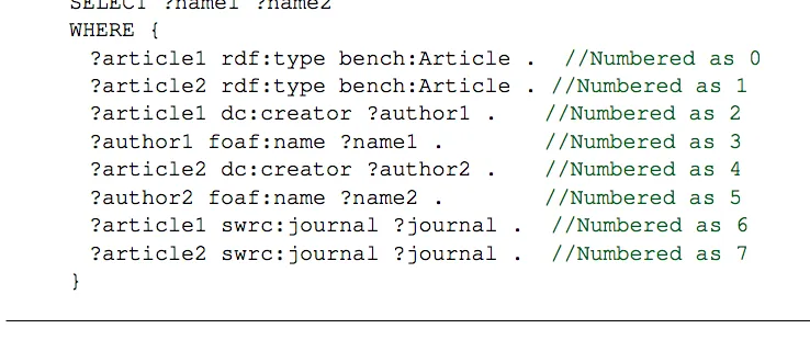
Mazumdar (2011) demonstrates how the join phase would iteratively process a certain SPARQL query shown in Figure 3.6. Figure 3.6 also shows how each of the different triple patterns are numbered for use later in the query planning stage.
FIGURE3.6: Mazumdar’s Example SPARQL Query (Mazumdar, 2011).
[image:49.596.113.499.86.355.2] [image:49.596.112.481.482.637.2]and 6 share the common variable ?article1, so they would be joined in the first Map/Reduce join pass.
FIGURE3.7: Mazumdar’s Query Execution Plan (Mazumdar, 2011).
The resulting output, with the completed join of patterns 0,2 and 6 highlighted in blue, is shown in Figure 3.8. The join phase would continue in this manner, joining all elements sharing a common variable via a single Map/Reduce task. According to Mazumdar (2011), using this method would take a further four iterations to produce the final join stage output. This would then serve as the input to the projection stage which performs the ’SELECT’ clause of the query shown in Figure 3.6, in this case outputting the request variables of ?name1 and ?name2.
FIGURE3.8: Mazumdar’s First Join Iteration (Mazumdar, 2011).
system evaluates which of the pre-split files are required as input for the job. Then, Husain et al. (2011) explain that the system implements an heuristic approach to find the optimum method to complete the query. This heuristic approach to finding the best query plan is what differentiates HadoopRDF from other implementations and, due to its ability to cut the number of Map/Reduce iterations, is a key driver of its performance (Goasdou ´e et al., 2013). The heuristics-based approach uses a greedy algorithm to determine the minimum numbers of jobs in which a set query can be completed. Once the appropriate plan has been generated, the system then runs the required number of jobs in a pre-determined order. The input for a certain job is the output from the previous job, with the original input being the required selection of split RDF files. If any joins are required on different variables, HadoopRDF processes them using iterative reduce-side joins. However, HadoopRDF will join any number of identical variables in a single pass in an effort to reduce the number of required passes (Husain et al., 2011).
Goasdou ´e et al. (2013) present an alternative Map/Reduce based RDF query system which borrows the idea of cliques from graph theory to perform certain queries in a highly efficient manner. They propose a system of two different clique-based query classifications. Firstly, they propose the 1-clique query, which are only those queries which join triples via a single common variable. Figure 3.9(a) shows a SPARQL query which, based on the single com-mon join variable ?x, would be classified as a 1-clique query. Figure 3.9(b) shows the graph representation of the same query, with each node being a single triple pattern, connected by their common join variable of ?x. To implement the 1-clique query via Map/Reduce Goasdou ´e et al. (2013) exploit their data replication strategy discussed in section 3.5. The strategy ensures that any triples which share at least one element are accessible on a single node. They are then able to exploit the ability of map side joins, highlighted in section 3.3.1, to perform joins on a single common key in a map only job, bypassing the costly shuffle/sort phase. Goasdou ´e et al. (2013) performed an analysis of real-world SPARQL queries taken from DBPedia before they designed the system. They observe that nearly 99% of queries from the real-world sample have the potential to be processed via a 1-clique query.
FIGURE3.9: Goasdoue 1-Clique Query (Goasdou ´e et al., 2013).
which would qualify as a central clique query. Figure 3.10(b) shows the same query repre-sented in graph form, illustrating how the two different collections of triple patterns are con-nected via a single element. To implement a central clique query in map/reduce, Goasdou ´e et al. (2013) exploit a map side join and then a reduce side join (discussed in section 3.3.2), to enable two different triple groups to be joined. For example the query from Figure 3.10 could be completed in one Map/Reduce iteration. Firstly as the query contains two distinct 1-clique queries, each of these would be completed in the map phase as before. Then the required additional join on the two separate patterns would be accomplished in the re-duce stage by setting the common variable as the intermediate key. Using this method, any number of different interconnected 1-clique patterns could be joined by using iterative Map/Reduce passes.
3.6.2 Presented Performance Results
This section will explore and compare relevant practical results presented in the literature detailed in the previous section.
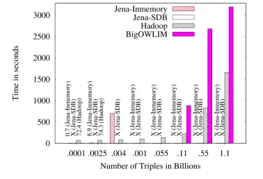
Mazumdar (2011) presents results from the developed solution on a 20 node cluster. To evaluate the performance, RDF data and SPARQL queries from the SP2 Benchmark were used. The SP2 Benchmark is a commonly used tool to assess the performance of triple-stores. It comprises a set of relatively simple SPARQL queries which are run across a variety of dataset sizes. Full details of SP2 are given by Schmidt, Hornung, Lausen, and Pinkel (2008). Figure 3.11 shows the results for the solution (Mazumdar, 2011). The results show that for even relatively simple queries running on a dataset size of 50 million triples, the solution takes up to 50 minutes to return a response.
FIGURE3.11: Mazumdar’s Performance Results (Mazumdar, 2011).
amount of triples is increased past 25 Million. They also show that Jena is unable to even process datasets of more than 100M triples. The results also show that the solution is able to perform a single SPARQL query on one billion triples in under one hour. Husain et al. (2011) also test the scalability of HadoopRDF by testing how the framework performs on datasets of up to 6.6 billion triples. They find that the system features a sub-linear increase in query time against dataset size, meaning that an increase in dataset size does not result in a proportional increase in the time taken to query it.
FIGURE3.12: Husain’s Performance Results (Husain et al., 2011).
Goasdou ´e et al. (2013) present results from their solution which is tested on an eight node cluster. As well as assessing their own work, they also compare it to the HadoopRDF system created by Husain et al. (2011). They are also using the LUBM Benchmark to test the upload and query performance of the system. Figure 3.13 shows the upload performance of the system on dataset sizes of one and two billion triples. The results show that the system required 257 minutes to upload one billion triples and the system failed to upload two billion triples over the eight node cluster.
[image:54.596.115.493.243.501.2]FIGURE3.13: Goasdoue’s Upload Performance Results(Goasdou ´e et al., 2013).
in 59 minutes. These results show that the solution presented by Goasdou ´e et al. (2013) has the best performing query stage of the current SPARQL over Hadoop processing solutions as detailed in section 3.6.
FIGURE3.14: Goasdoue’s Query Performance Results(Goasdou ´e et al., 2013).
3.7
Limitations Of Existing Hadoop RDF Solutions
SPARQL queries from the LUBM or SP2 benchmarks. None give details on how the sys-tems cope when required to perform large numbers of joins which a complex SPARQL query would entail. In addition, none of the current solutions explore the possibility of grouping common joins from different unique SPARQL queries together to save on re-computation.
The following two sections explore two of the main limitations that the current systems share.
3.7.1 Hadoop Joining Strategies
Many of the existing projects which tackle processing RDF over Hadoop rely on the slower reduce side join, meaning that they would require many iterations to processes complex queries. Few attempts have looked at the possibility of a map-side or broadcast join to create highly optimised systems. The work presented by Mazumdar (2011), Rohloff and Schantz (2010), Husain et al. (2011) and Kulkarni (2010) all perform any required joins via a series of cascade reduce-side joins. As described in section 3.3.3, cascade joins involve a lot of data transfer over the network as well as incurring multiple JVM initialisation stages, both of which will lead to poor performance. From the currently available literature, only one solution has been developed which attempts to use a map-side join when processing SPARQL queries. This is the clique-based approach presented by Goasdou ´e et al. (2013). This approach uses a map-side method to join triples which share a common element but falls back to a reduce side method to join additional elements. There appear to be no available solutions which utilise the highly efficient broadcast join method.
3.7.2 Data Upload Stages
Many of the current solutions rely on pre-processing of the data to enable faster querying at a later date. However these data upload stages often change the structure of the data, thus removing the characteristic triple format and element order of the RDF data to be stored. For example the solution presented by Husain et al. (2009) split the original RDF dataset into different files based on the predicate, meaning that the files would have to be reconstituted if the user wanted to extract the complete original RDF dataset. In the example presented by Goasdou ´e et al. (2013), the order of the RDF elements is altered for each of the three data replications, meaning that the user would have to re-convert the data back to its original order of subject, predicate and object. The data upload stage presented by Goasdou ´e et al. (2013) also has a further limitation, in that it can only be used to join dataset sizes less then the size of a HDFS block; by default this is 64MB.
These approaches would need additional Map/Reduce jobs to convert the data back into the original RDF format. None of the currently available literature explores the possibility of storing and querying RDF data over Hadoop in its native format. There may very well be good performance-related reasons for this, but as all the upload stages presented in the literature take considerable time, the possibility of not requiring one should be explored.
3.8
Possibility Of A Highly Optimised Solution
Analysis Of Current Jena TDB
Implementation
4.1
Current Implementation
This chapter will introduce and analyse the pre-existing approach used to assess the quality of medical data using linked data technologies. This approach was developed by Dr David Corsar and Dr Laura Moss and full details are given by Corsar et al. (2012) and Moss, Corsar, and Piper (2012).
Corsar et al. (2012) state that this framework can be broken down into three key stages: firstly, pre-existing medical data is converted into RDF data and stored in Jena TDB. Sec-ondly, the data can be annotated with provenance information, such as the specification of the machines which recorded the data. Lastly, a data-checking component assesses the quality via a series of SPARQL rules. Figure 4.1 shows the complete framework. The most important of these steps is the data checking stage, which according to Corsar et al. (2012), comprises a series of SPARQL queries which test various qualities of the data, including checks on acceptable data ranges and missing data points. If a potential error is found the system will annotate it with one of two different states based on the level of confidence that it is truly an error. The two states are ’Possible Error’ and ’Probable Error’ (Corsar et al.,
2012). The function of the data checking stage is to highlight any potential errors in the dataset to the user before the data is utilised for other purposes.
FIGURE4.1: Current Approach For Checking Medical Data (Corsar et al., 2012).
4.2
Limitations of Existing Solution
While the current framework functions correctly in the detection of errors, it suffers from two main performance issues, details of which are given in the papers describing the framework. Firstly Corsar et al. (2012) explain that their original method of using Jena TDB took over six hours to upload 1.6 Million triples. Secondly, Moss et al. (2012) explain how the framework, when working on an RDF dataset comprising 609,168 triples, took over 150 minutes to return a response for a single SPARQL query. Both these performance issues are related to the same Semantic Web component of the framework; Jena TDB.
4.3
Current Implementation Performance Analysis
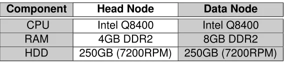
To assess the real-world performance of the Jena-based framework, it was benchmarked against a range of RDF dataset sizes. Hardware and software specifications of the machine on which the benchmarks were run can be seen in section 6.1.1. Both the upload and query time for the Jena implementation were benchmarked.
A more detailed and comparative analysis of the Jena framework can be found in section 7.5.
4.3.1 Upload Time
Figure 4.2 shows the upload performance of Jena TDB across a range of data set sizes. As the results show, the upload performance of Jena TDB is poor once the dataset size increases past 32 million triples, as Jena took 157 minutes to upload 64 million triples. While this upload performance is not as poor as the claims made by Corsar et al. (2012) and Moss et al. (2012), direct comparisons between the two results is impossible due to the lack of knowledge about the test environment and datasets used by Corsar et al. (2012) and Moss et al. (2012). However both results due suggest that Jena is not able to cope with storage demands made by the massive potential volumes of NHS RDF data.
4.3.2 Query Time
FIGURE4.2: Jena TDB Upload Performance
FIGURE4.3: Jena TDB Query Performance
4.3.3 Analysis
machine. This machine is detailed in section 6.1.1. The results for the upload and query stages produce unsatisfactory results when the number of triples is increased to 64M. In-deed Jena was not able to return a result when the dataset size was increased to 128 million triples. Neither the upload nor query performance is as poor as (Corsar et al., 2012) and (Moss et al., 2012) found, however this could be explained by a performance disparity between the underlying machines used in the test. .
4.4
The Need For A New Framework
Hadoop Implementation and
Algorithm Design
As shown in Chapter 4, there is a clear need to produce a new framework that can cope with the potential volume of NHS RDF data. This chapter will detail how this new framework was first designed and then implemented.
5.1
Structure and Distribution Of The Real-World Medical Data
For any new framework to be designed, real-world medical data was required. Due to ethical and privacy reasons it was not possible to have access to large volumes of real medical data. However, three anonymised datasets were provided by the University Of Glasgow. The datasets all contain neurological data from the BrainIT project (Chambers et al., 2009). The datasets contain information regarding neurological readings taken from patients, along with information regarding the machines and sensors which produced these values. The provided datasets represent a small period of time for three different patients and combined they contain 7,933,649 RDF triples. More medical data was synthetically generated for use in later tests, details of this process can be found in section 5.2.
The rest of this section will explore the structure and distribution of the three real-world medical data sets.
5.1.1 Subject, Predicate and Object Distribution
To better understand the distribution of the data, the number of unique RDF Subjects, Pred-icates and Objects were obtained using a simple Map/Reduce job. The results of which can be seen in table 5.1.
RDF Element Number Of Elements
Subject 1,523,106
Predicate 61
Object 1,711,702
TABLE5.1: Subject, Predicate and Object Distribution
The results show that only 61 unique predicates are used throughout all of the datasets. Further, it can be seen that the number of unique subjects and objects are closely matched. It also shows that compared to the total number of triples (7,933,649), many of the subjects and objects are replicated numerous times.
5.1.2 Distinct Triple Group Distribution
As will be explained in section 5.3, all of the original SPARQL queries join distinct groups of triples, which are linked by a common theme. Broadly, the distinct groups of triples are related to two things: patient recording values and permitted value ranges. For any possible optimisations for later queries, knowledge of the distribution of these triple groups would be required. In order to explore the distribution of these groups a Map/Reduce algorithm was devised that assessed the number of members in set triple groups. This was then run against the same three medical RDF datasets, grouping the triples into one of three groups. The groups were ?range, ?obs and ?cs and were chosen to reflect the triple groups used in the SPARQL queries. The result is shown in table 5.2.
Triple Group Name Number Of Elements
?obs 3,426,188
?range 518
?cs 446
The results show that the distribution of the triple groups is massively skewed towards the ?obs group. The ?obs group has 3,426,188 unique triple instances, which when compared with the total number of triples in the dataset (7,933,649) shows the ?obs group comprises a large proportion of the total triples. Both the ?range and ?cs groups contain very few instances.
5.2
Data Generation
Due to not having access to large volumes of medical data, it became apparent that data would have to be synthetically generated. As the framework needed to be tested against massive datasets, one billion triples were generated. To produce the new data, a Map/Re-duce algorithm was developed which generated new RDF data based upon an input of real world medical RDF data. The algorithm retains the structure and distribution from the real world data, but inserts new randomly generated values for the variable triple elements. The algorithm exploits knowledge of the data so that it does not alter triples which are constant across all datasets, for example the from the ?range triple group.
To ascertain that the newly generated data matched the structure, distribution and triple group distr