Element Free Gelerkin Method for 2 D Potential Problems

http://dx.doi.org/10.4236/am.2015.61015

How to cite this paper: Firoozjaee, A.R., Hendi, E. and Farvizi, F. (2015) Element Free Gelerkin Method for 2-D Potential Problems. Applied Mathematics, 6, 149-162. http://dx.doi.org/10.4236/am.2015.61015

Element Free Gelerkin Method for 2-D

Potential Problems

Ali Rahmani Firoozjaee*_{, Ehsan Hendi, Farzad Farvizi}

Faculty of Civil Engineering Department, Babol University of Technology, Babol, Iran Email: *[email protected]

Received 20 November 2014; accepted 2 December 2014; published 16 January 2015

Copyright © 2015 by authors and Scientific Research Publishing Inc.

This work is licensed under the Creative Commons Attribution International License (CC BY).

http://creativecommons.org/licenses/by/4.0/

Abstract

A meshfree method namely, element free Gelerkin (EFG) method, is presented in this paper for the solution of governing equations of 2-D potential problems. The EFG method is a numerical method which uses nodal points in order to discretize the computational domain, but where the use of connectivity is absent. The unknowns in the problems are approximated by means of connectivity- free technique known as moving least squares (MLS) approximation. The effect of irregular dis-tribution of nodal points on the accuracy of the EFG method is the main goal of this paper as a complement to the precedent researches investigated by proposing an irregularity index (II) in order to analyze some 2-D benchmark examples and the results of sensitivity analysis on the pa-rameters of the method are presented.

Keywords

Element Free Galerkin (EFG) Method, Potential Problems, Moving Least Squares Approximation, Irregular Distribution of Nodal Points, Irregularity Index

1. Introduction

Partial differential equations arise in connection with various physical and geometrical problems in which the functions involved depend on two or more independent variables, usually on time t and on one or several space variables [1]. A potential problem is one of the most important partial differential equations in engineering ma-thematics, because it occurs in connection with gravitational fields, electrostatics fields, steady-state heat con-duction, incompressible fluid flow, and other areas [1].

Mesh based numerical methods, such as finite element method (FEM) and boundary element method (BEM), have been the primary numerical techniques in engineering computations. In spite of the positive points of the

finite element method, it still suffers from high preprocessing time, low accuracy of stresses, difficulty in incor-porating adaptivity and it is also not an ideal tool for certain classes of problems, e.g. large deformations, ma-terial damage, crack growth, and moving boundaries [2] [3]. Therefore, meshless or meshfree methods are an ideal choice for these problems, because only a set of nodes is required for the problem domain discretization.

In the past few decades, a variety of new meshless methods have been developed, including the smoothed particle hydrodynamics (SPH) method [4], the finite point method (FPM) [5], the diffuse element method (DEM) [6], the element free Galerkin (EFG) method [7], the point interpolation method (PIM) [8], the hp clouds method [9], the partition of unity method (PUM) [10], the meshless local Petrov-Galerkin (MLPG) method [11], the lo-cal point interpolation method (LPIM) [12], the discrete least squares meshless (DLSM) method [13], the boun-dary point interpolation method (BPIM) [14], and the meshless method with boundary integral equations [15]- [18].

Recently several meshless methods are proposed in order to solve potential problems. The improved EFG method [19] based on the improved MLS approximation is used to solve 2-D potential problems. The method of fundamental solution (MFS), in which the desingularization technique is used to regularize the singularity and hyper singularity of the kernel functions, is applied to solve potential problems [20]. The discrete least squares meshless method with extra Gauss points is suggested for the solution of elliptic partial differential equations [21]. Singh and Singh used EFG method to solve 2-D potential flow problems [22] with regular distribution of nodal points.

The element free Galerkin (EFG) method that was developed by Belytschko et al. [7], is one of the most commonly used meshless methods and is based on the earlier version of diffuse element method [6]. In the EFG method, moving least squares (MLS) shape functions are used for the approximation of the field variables [23]; a background cell is used for numerical integration and Lagrange multipliers or penalty method is used for the imposition of essential boundary conditions.

The element free Galerkin method is presented in this paper to solve potential problems, and the effect of ir-regularity distribution of nodal points by using a proposed irir-regularity index (II) that was not considered in the previous researches for the EFG method, is investigated. In what follows, the construction of MLS shape func-tions is first explained. EFG method for discretization of the governing differential equation is then explained. Several 2-D potential problems are solved using the proposed method; sensitivity analysis on the parameters of the proposed method is also carried out, and the results are presented.

2. MLS Approximation

2.1. MLS Interpolants Function

MLS is a very important component of the element free Galerkin (EFG) method for the approximation of the field variables. The MLS approximation uhof a scalar function u at point x is given as

( )

( ) ( )

T

( ) ( )

1

m h

i i i

u p a P a

=

=

∑

=

x x x x x (1)

where P(x) is a polynomial basis function of the spatial coordinates, m is the number of monomial terms in the basis function, and a x

( )

is a vector of coefficients given by

( )

(

( ) ( )

( )

)

T

1 , 2 , , m

a x = a x a x  a x (2)

The polynomial basis function P(x) is built from Pascal’s triangle and pyramid for 2- and 3-D problems, re-spectively. In 2-D problems, linear and quadratic basis functions are given as

( ) (

) (

)

T _{1, , 3 linear basis}

P x = x y m= (3)

( )

(

)

(

)

T 2 2

1, , , , , 6 quadratic basis

P x = x y xy x y m= (4)

(

)

( ) ( )

2

(

)

( ) ( ) ( )

2

1 1 1

n n m

h

I I I i i i I

i i i

J W u u W p a u

= = =

 

 

= − _ − _ = − _ ⋅ − _

 

∑

x x x x

∑

x x

∑

x x x (5)

where W

(

x x− I

)

is the weight function of node xI at a point x which for simplicity it will be stated as

( )

I

W x .

Equation (5) using vector notation can be written as:

(

)

T

( )(

)

J= pa−u W x pa−u (6)

The minimum of J with respect to a x

( )

is found by

0

J a

∂ ₌

∂ (7)

This leads to the following system of linear equations

( ) ( )

( )

A x a x =B x U (8)

Here A x

( )

and B x

( )

are

(

m m×

)

and

(

m n×

)

matrices, respectively, and are given as

( )

( )

( ) ( )

T

1

n

i i i i

A W p p

=

=

∑

x x x x (9)

( )

1

( ) ( )

1 , 2( )

( )

2 , 3

( ) ( )

3 , , n

( ) ( )

n

B x = W x P x W xP x W x P x W x P x _ (10)

And U is

(

n×1

)

vector and is given as

[

]

T

1, 2, 3, , n

U= u u u u (11)

( )

a x can be found using Equation (8);

( )

1

( ) ( )

a x =A− x B x U (12)

Putting a x

( )

from Equation (12) into Equation (1) leads to

( )

T

( ) ( ) ( )

1

( )

( )

1

n h

i i i

u P A− B U φ U ϕ u

=

= = =

∑

x x x x x x (13)

where φ

( )

x is a vector of shape functions. The first derivative of the shape functions with respect to the spatial coordinates is also required for the numerical implementation and is given as

(

)

T 1 T 1 1

,i P A B,i P A B,i A B,i

φ ₌ − ₊ − ₊ −

(14)

where

1 1

,i ,i

A = −A A A− − (15)

and the index after the comma is a spatial derivative.

2.2. Weight Function

Weight function is an important part of the MLS approximation. There are no predefined rules to select the weight function for a particular application, but the weight function that could be used for meshless methods should have the following properties:

1) Its value should be maximized at the node and decrease with the distance from the node. 2) Smooth and non-negative.

Influence domain of a nodal point is a very important concept in meshless methods, as it determines the re-gion in which it has influence. The size of influence domain for a node i is dw=dmaxci, where dmax is a scal-ing parameter and ci is determined by searching for enough neighbor nodes such that matrix A in Equation (8)

is invertible. In regular distribution of nodal points ci can be chosen as the distance between two neighboring

nodes. In this paper, the cubic spline weight function is used;

( )

2 3

2 3

2 1

4 4 for

3 2

4 4 1

4 4 for 1

3 3 2

0 for 1

d d d

W d d d d d

d

 − + ≤

  

=_ − + − < ≤



 >



(16)

where d =

(

x−x_i

)

d_w is the distance between node xi and point of interest

x

. Weight function

deriva-tives with respect to the spatial coordinates are also required for the shape function derivaderiva-tives as given in Equa-tion (14) and are given as follows [2]:

2

2

1 8 12 for

2

d 1

4 8 4 for 1 2 d

0 for 1

d d d

W

d d d

d d − + ≤   

= − +_ − < ≤



 >



(17)

3. EFG Method for Potential Problems

3.1. 2-D Potential Formulation

Consider a Poisson’s partial differential equation in a two dimensional domain Ω bounded by Γ;

( )

2

, 0, in

u g x y

∇ + = Ω (18)

where g x y

( )

, is a source term. On one part of the boundary, Γu is the Dirichlet boundary condition, and on

the other part, Γq is the Neumann boundary condition.

, on u

u=u Γ (19)

, on q

u q n

∂ _{= Γ}

∂ (20)

where n is the outward normal vector to the boundary.

3.2. Enforcement of Essential Boundary Condition

The MLS shape functions do not satisfy the Kronecker delta property, i.e. φ_i

( )

x_j ≠δ_ij, and are termed as ap-proximants instead of interpolants. The values obtained from the MLS approximation are therefore, not the same as the nodal values, i.e. uh

( )

xi ≠ui, and are known as nodal parameters. This leads to some difficulties in

im-position essential boundary condition in contrast to conventional FEM [2].

In this paper, the penalty method is used to enforce the essential boundary condition. The use of penalty me-thod produces system of equations of the same dimension that FEM produces for the same number of nodes, and the modified stiffness matrix is still positively defined; moreover, the symmetry and the bandedness of the sys-tem matrix are preserved [2].

In the EFG method, the essential boundary condition has the form

( )

, on

n

i i u i

u u

φ = Γ

where u x

( )

is the prescribed potential on the boundary.

Consider the problem stated in Equation (18), a penalty factor is applied to penalize the difference between the potential of the MLS approximation and the prescribed potential on the essential boundary [2]. The con-strained Galerkin weak form uses the penalty method and with substituting the expression of MLS approxima-tion of Equaapproxima-tion (13) can then be posed as

d d d d 0

q u u

i i

i q i u i u i

u u

q u ud g

x x y y

φ φ _{φ α φ α φ φ}

Ω Γ Γ Γ Ω

∂ ∂

 ∂ ∂ 

− _ + _ Ω + Γ + Γ − Γ + Ω =

∂ ∂ ∂ ∂

 

∫∫

∫

∫

∫

∫∫

(22)

where α=

(

α α1, 2,,αk

)

is a diagonal matrix of the penalty factor that k=2 for 2-D case. The penalty fac-tor α_i

(

1,,α_k

)

can be a function of the coordinates, and it can be different from one another. Although in practice the identical constant of a large positive number is assigned for penalty factor, which can be chosen by following method [2]

(

)

4 13

1.0 10 max diagonal element in the stiffness matrix

α _{= ×} − _×

(23)

The final system of equation of the EFG formulation with penalty method is

K Kα u F Fα

 +  = +

  (24)

where d j j i i ij K

x x y y

φ φ

φ φ

Ω

∂ ∂

∂ ∂ 

= _ + _ Ω

∂ ∂ ∂ ∂

 

∫∫

(25)

q

d d

i i q i

F qφ φg

Γ Ω

=

_∫

Γ +

_∫∫

Ω (26)

The additional matrix Kα is the global penalty matrix assembled using the nodal matrix defined by

d

u

ij i j u

Kα α φ φ

Γ

=

_∫

Γ (27)

And the vector Fα is caused by the essential boundary condition that its nodal vector has the form

d u

i i u

Fα α φu

Γ

=

_∫

Γ (28)

4. Irregularity Index (II)

To demonstrate the efficiency and accuracy of the EFG method in dealing with irregular distribution of nodal points, following irregularity index (II) is proposed in this paper

min

max II r

r

= (29)

where rmax and rmin are the maximum and minimum distances between nodal points, respectively, that are located in circular local domain such that each local domain includes at least 5 nodal points. The interval of the proposed index is 0≤ ≤II 0.5, in which 0 indicates fully irregular and 0.5 indicates fully regular distribution of nodal points.

5. Numerical Examples

5.1. 2-D Poisson’s Equation with Mixed Boundary Conditions Consider the following 2-D Poisson’s equation

( ) ( )

2 2

2 2 cos π cos π , 0 1, 0 1

u u

x y x y

x y

∂ ∂

+ = ≤ ≤ ≤ ≤

∂ ∂ (30)

with the following Dirichlet and Neumann boundary conditions

( )

2

( )

( )

2

( )

1 1

, 0 cos π , 0, cos π

2π 2π

u x = − x u y = − y (31)

( )

1, 0,

( )

,1 0

u u

y x

x y

∂ ∂

= =

∂ ∂ (32)

the analytical solution of the aforementioned Poisson’s equation is

( ) ( )

2

1

cos π cos π 2π

exact

u = − x y (33)

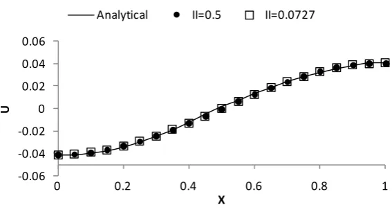
[image:6.595.238.391.371.523.2]

The above-mentioned problem is solved using two different sets of 81 distributed nodes. In all of these cases, the polynomial basis function is considered as PT =[1 ]x y and the ratio of influence domain is considered 3. The regular and irregular distribution of 81 nodal points for this problem is shown in Figure 1 and Figure 2. The analytical and EFG solution on a mesh of 81 nodal points with 96 and 1152 Gauss points along x axis are shown in Figure 3 and Figure 4, respectively, to assess the effect of number of Gauss points on the solution accuracy.

[image:6.595.240.389.551.706.2]

Figure 1.Nodal distribution on a rectangular domain with II = 0.5.

Figure 2.Nodal distribution on a rectangular domain with II = 0.0727. 0.0

0.1 0.2 0.3 0.4 0.5 0.6 0.7 0.8 0.9 1.0

0.0 0.5 1.0

0.0 0.1 0.2 0.3 0.4 0.5 0.6 0.7 0.8 0.9 1.0

[image:7.595.173.455.82.228.2]

Figure 3.Results obtained by analytical and EFG method at y = 0.2with 96 Gauss points.

Figure 4. Results obtained by analytical and EFG methodat y = 0.2 with 1152 Gauss points.

There are different parameters in the EFG method that affect the obtained results. In this paper a sensitivity analysis is carried out on these parameters. Number of nodal points, number of Gauss points, ratio of influence domain, number of monomial terms in the basis function, and the type of weight function, are the parameters that are analyzed. For the sensitivity analysis the following error norm has been used

1 0

1 n

exact num

i i

i n

exact i i

u u

e

u =

=

−

=

∑

∑

(34)

where uiexact and num i

u is the quantity of analytical solution and numerical solution, respectively. For the sensi-tivity analysis, one of the parameters is changed while the others are constant. The result of this analysis is shown in Tables 1-10, and the computational time is presented.

The results of Table 1 indicate that the errors are dramatically reduced with increasing the number of nodal points while they get nearly constant when more nodal points are added. These results are also used to evaluate the convergence rate of the method with respect to nodal points and the results are shown in Figure 5.

The results of Table 2 and Table 3 quantitatively emphasize the rule of Gauss points on the accuracy of the EFG method and demonstrate high accuracy and low sensitivity of the proposed method in dealing with irregu-lar distribution of nodal points.

This problem is solved here with different values of irregularity index to present the effect of irregularity dis-tribution of nodal points. This analysis is done by using a proposed index that is shown in Table 4 and a con-vergence rate is also demonstrates the obtained results in Figure 6. These results indicate the convergent beha-vior of the method as expected.

-0.06 -0.04 -0.02 0 0.02 0.04 0.06

0 0.2 0.4 0.6 0.8 1

U

X

Analytical II=0.5 II=0.0727

-0.06 -0.04 -0.02 0 0.02 0.04 0.06

0 0.2 0.4 0.6 0.8 1

U

X

[image:7.595.172.456.259.412.2]

Table 1. The effect of number of nodal points on the error norm with 480 regular Gauss points.

Number of nodal points 25 36 64 81

x

∆ 0.250 0.200 0.143 0.125

0

e 0.3944 0.0730 0.0031 0.0029

CPU TIME (Sec) 0.6708 0.7800 0.8580 0.9572

Table 2. The effect of number of Gauss points on the error norm with 81 regular nodal points.

Number of Gauss points 96 320 480 1152

0

e 0.0153 0.0032 0.0029 0.0022

CPU TIME (Sec) 0.6084 0.7800 0.9672 1.6848

Table 3. The effect of number of Gauss points on the error norm with 81 irregular nodal points.

Number of Gauss points 96 320 480 1152

0

e 0.3273 0.2289 0.1323 0.0577

CPU TIME (Sec) 1.3193 2.2932 2.3868 4.5396

Table 4. The effect of irregularity of nodal points on the error norm with 81 irregular nodal points.

Irregularity Index (II) 0.5 0.0727 0.0143 0.0012

0

e 0.0002 0.0577 0.0991 0.1907

CPU TIME (Sec) 1.6848 4.5396 0.9984 1.6068

Table 5.The effect of ratio of influence domain on the error norm with 81 regular nodal points.

Ratio of influence domain 1.12 2 3 4.8 6.4

0

e 0.0112 0.0026 0.0007 0.1156 0.6371

CPU TIME (Sec) 0.3276 0.7176 1.5912 4.4928 7.5660

Table 6. The effect of ratio of influence domain on the error norm with 81 irregular nodal points.

Ratio of influence domain 1.12 2 3 4.8 6.4

0

e 0.7114 0.1583 0.0577 0.0134 0.0025

CPU TIME (Sec) 1.2168 1.5756 4.5396 13.3536 22.3237

Table 7. The effect of number of monomial terms in basis function on the error norm (regular).

The number of monomial terms in the basis function 0 1 2

0

e 0.0029 0.0007 0.0006

CPU time (Sec) 1.2792 1.5912 2.3868

Table 8.The effect of number of monomial terms in basis function on the error norm (ırregular).

The number of monomial terms in the basis function 0 1 2

0

e 0.0267 0.0577 0.1645

Table 9.The effect of the type of weight function on the error norm with 81 regular nodal points.

Type of weight functions Cubic spline Quartic spline Exponential

0

e 0.0006 0.0016 0.0070

CPU time (Sec) 2.3868 2.4180 2.3556

Table 10.The effect of the type of weight function on the error norm with 81 irregular nodal points.

Type of weight functions Cubic spline Quartic spline Exponential

0

e 0.0577 0.1428 0.2116

CPU time (Sec) 4.5396 3.2136 4.1340

Figure 5. Convergence rate of the method with respect to nodal points.

Figure 6.Convergence rate of the method with respect to irregularity index.

The problem is solved again on a mesh of 81 regularly and irregularly distributed of nodal points with differ-ent ratio of influence domain and 1152 Gauss points. The effect of this parameter is investigated in Table 5 and Table 6. The values of this ratio in Table 6 vary in the same way as Table 5 to have a better comparison be-tween them. The results of Table 5 demonstrate that the appropriate interval of ratio of influence domain in reg-ular distribution of nodal points is 2 - 3, while it is obvious from Table 6 that the errors are decreased by in-creasing this ratio.

The number of monomial terms in basis function is the other parameter that can affect the performance of the EFG method. In this case, the problem domain is discretized with 81 regular and irregular nodal points with 1152 Gauss points. The ratio of influence domain in Table 7 and Table 8 is considered 3 to have a better com-parison between them.

y = 7.0528x + 3.8223

-4 -3.5 -3 -2.5 -2 -1.5 -1 -0.5 0 0.5 1

-0.95 -0.85 -0.75 -0.65 -0.55

Lo

g (e

0

)

Log (Δx)

y = -0.9913x - 3.3128

-4 -3.5 -3 -2.5 -2 -1.5 -1 -0.5 0

-3 -2.5 -2 -1.5 -1 -0.5 0 0.5

L

o

g (

e0

)

According to the results of Table 7 and Table 8, the errors are diminished by increasing the number of mo-nomial terms in basis function in regular distribution of nodal points, however, this effect is opposite in irregular distribution of nodal points because the higher number of monomial terms, the more nodal points are acquired in a favorable influence domain.

The other parameter that affects the solution’s accuracy of the EFG method is the type weight function. In order to investigate this effect, the problem domain is discretized again with 81 regular and irregular meshes of nodes with 1152 Gauss points and three types of weight functions that are considered. It is also notable that the ratio of influence domain in both cases is considered 3.

It can be concluded from Table 9 and Table 10 in both cases, the solution’s accuracy obtained by cubic spline is more desirable than the other weigh functions.

5.2. Poisson’s Equation with Dirichlet Boundary Conditions on a Torus [19]

The second example is a 2-D Poisson’s equation with Dirichlet boundary conditions on the torus. The equation is

2 2

2 2

d d

4 0 , 0 2π

d d

u u

a r b

x + y − = < < < <θ (35)

with the following boundary conditions

( )

, 0

u aθ = (36)

( )

, 0

u bθ = (37)

and the analyticalsolutionofthisproblemis

( )

(

2 2

) (

2 2

)

log log ,

log log

r a

u r r a a b

a b

θ = − − − _ − _

−

  (38)

here, a=1 and b=2 are assumed. The regular distribution of nodal points is shown in Figure 7. The above- mentioned problem is solved using two different sets of 460 distributed nodes that are shown in Figure 7 and Figure 8. The analytical and numerical solutions along r direction at any angle with 460 nodal points are plotted in Figure 9 and the ratio of influence domain is considered 3 for this problem again.

5.3. Flow over a Circular Cylinder

In this section, flow over a circular cylinder is considered. Such a flow can be generated by adding a uniform flow, in the positive x direction to a doublet at the origin directed in the negative x direction. The geometry of the example is shown in Figure 10 and the governing equation of that is as follows:

2 2

2

2 2 0, in

x y

φ φ

φ ∂ ∂

∇ = + = Ω

[image:10.595.245.385.529.707.2]

∂ ∂ (39)

Figure 7. Nodal distribution on a tours domain with II = 0.3862.

-2 -1.5 -1 -0.5 0 0.5 1 1.5 2

[image:11.595.200.430.66.668.2] [image:11.595.241.391.86.236.2]

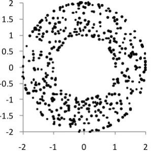
Figure 8. Nodal distribution on a tours domain with II = 0.0114.

Figure 9. Results obtained by analytical and EFG method alongr direction at any angle.

8

8 2 1m

u s

=

Figure 10. Flow over acircular cylinder.

and the exact solution is

(

2 2

)

1

x u

x y

φ₌  ₊ 

 + 

 

(40)

where u is the fluid’s velocity. Due to the symmetry, only the one-quarter of the problem domain is consi-dered. This domain with its boundary condition is shown in Figure 11.

-2 -1.5 -1 -0.5 0 0.5 1 1.5 2

-2 -1 0 1 2

-0.6 -0.5 -0.4 -0.3 -0.2 -0.1 0

1 1.2 1.4 1.6 1.8 2

U

r

[image:11.595.212.415.273.466.2]

The above-mentioned problem is solved using three different sets of 241 distributions of nodal points with 962 Gauss points. It is notable that the ratio of influence domain in all cases is considered 3 and the distribution of nodal points with different values of irregular index is shown in Figure 12-14. The analytical and the EFG solutions along y axis are shown in Figure 15.

6. Conclusion

A meshless method namely element free Galerkin (EFG) method is presented in this paper. In order to investigate the performance and accuracy of the method, some 2-D potential problems on regular and irregular distribution

1 4

4

0

y

φ

∂ ₌ ∂

1

x

φ

∂ ₌ ∂

0

y

φ

∂ ₌ ∂

0

n

φ

∂ ₌ ∂

0

φ=

[image:12.595.239.387.198.329.2]

Figure 11. Boundary condition of the flow over a circular cylinder.

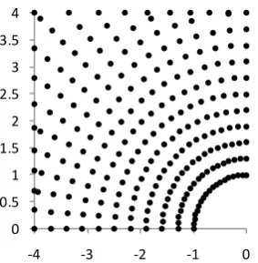
Figure 12. Nodal distribution of flow over a circular cylinder with II = 0.49999.

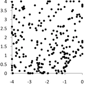
Figure 13. Nodal distribution of flow over a circular cylinder with II = 0.02323.

0 0.5 1 1.5 2 2.5 3 3.5 4

-4 -3 -2 -1 0

0 0.5 1 1.5 2 2.5 3 3.5 4

[image:12.595.244.385.362.504.2] [image:12.595.244.386.540.685.2]

[image:13.595.243.384.86.227.2]

Figure 14. Nodal distribution of flow over a circular cylinder with II = 0.00289.

Figure 15. Results obtained by analytical and EFG method at x = −1.0.

of nodal points by using a proposed irregularity index (II) are analyzed and compared with the exact solution. A sensitivity analysis on the parameters of the EFG method is also carried out. From above analysis, it can be in-ferred that the errors are dramatically reduced by increasing the number of nodal points and Gauss points while they get nearly constant when more of them are added. It is also notable that the appropriate ratio of influence domain has been found to be 2 - 3 for regular mesh of nodal points, and in irregular mesh of nodal points, the errors are converged by increasing this ratio. Increasing the number of monomial terms in basis function is another factor that can improve the accuracy of the EFG method in regular distribution of nodal points while this effect is contradictory in comparison with irregular distribution of nodal points. The effect of using different type of weight functions is another parameter considered and the results indicate better performance of the me-thod in using cubic spline weight function. Finally, it can be concluded that EFG meme-thod can be used to solve problems on irregular mesh of nodes with admissible performance.

References

[1] Kreyszig, E. (2010) Advanced Engineering Mathematics. Wiley, Hoboken.

[2] Liu, G.R. and Gu, Y. (2005) An Introduction to Meshfree Methods and Their Programming, Vol. 1. Springer, Berlin.

[3] Zhuang, X. (2010) Meshless Methods: Theory and Application in 3D Fracture Modelling with Level Sets. Durham University, Durham.

[4] Monaghan, J.J. (1988) An Introduction to SPH. Computer Physics Communications, 48, 89-96.

http://dx.doi.org/10.1016/0010-4655(88)90026-4

[5] Onate, E., et al. (1996) A Finite Point Method in Computational Mechanics. Applications to Convective Transport and Fluid Flow. International Journal for Numerical Methods in Engineering, 39, 3839-3866.

http://dx.doi.org/10.1002/(SICI)1097-0207(19961130)39:22<3839::AID-NME27>3.0.CO;2-R

[6] Nayroles, B., Touzot, G. and Villon, P. (1992) Generalizing the Finite Element Method: Diffuse Approximation and Diffuse Elements. Computational Mechanics, 10, 307-318. http://dx.doi.org/10.1007/BF00364252

0 0.5 1 1.5 2 2.5 3 3.5 4

-4 -3 -2 -1 0

-2.5 -2 -1.5 -1 -0.5 0

0 1 2 3 4

ϕ

Y

[image:13.595.187.445.262.399.2]

[7] Belytschko, T., Lu, Y.Y. and Gu, L. (1994) Element-Free Galerkin Methods.International Journal for Numerical Me-thods in Engineering, 37, 229-256. http://dx.doi.org/10.1002/nme.1620370205

[8] Liu, G.R. and Gu, Y. (2001) A Point Interpolation Method for Two-Dimensional Solids. International Journal for Numerical Methods in Engineering, 50, 937-951.

http://dx.doi.org/10.1002/1097-0207(20010210)50:4<937::AID-NME62>3.0.CO;2-X

[9] Liszka, T.J., Duarte, C.A.M. and Tworzydlo, W.W. (1996) hp-Meshless Cloud Method. Computer Methods in Applied Mechanics and Engineering, 139, 263-288. http://dx.doi.org/10.1016/S0045-7825(96)01086-9

[10] Babuška, I. and Melenk, J.M. (1997) The Partition of Unity Method. International Journal for Numerical Methods in Engineering, 40, 727-758. http://dx.doi.org/10.1002/(SICI)1097-0207(19970228)40:4<727::AID-NME86>3.0.CO;2-N

[11] Atluri, S. and Zhu, T. (1998) A New Meshless Local Petrov-Galerkin (MLPG) Approach in Computational Mechanics.

Computational Mechanics, 22, 117-127. http://dx.doi.org/10.1007/s004660050346

[12] Gu, Y. and Liu, G.R. (2001) A Local Point Interpolation Method for Static and Dynamic Analysis of Thin Beams.

Computer Methods in Applied Mechanics and Engineering, 190, 5515-5528.

http://dx.doi.org/10.1016/S0045-7825(01)00180-3

[13] Rahmani Firoozjaee, A. and Afshar, M.H. (2011) Discrete Least Squares Meshless (DLSM) Method for Simulation of Steady State Shallow Water Flows.Scientia Iranica, 18, 835-845. http://dx.doi.org/10.1016/j.scient.2011.07.016

[14] Gu, Y. and Liu, G. (2002) A Boundary Point Interpolation Method for Stress Analysis of Solids.Computational Me-chanics, 28, 47-54. http://dx.doi.org/10.1007/s00466-001-0268-9

[15] Liew, K., Cheng, Y. and Kitipornchai, S. (2007) Analyzing the 2D Fracture Problems via the Enriched Boundary Ele-ment-Free Method. International Journal of Solids and Structures, 44, 4220-4233.

http://dx.doi.org/10.1016/j.ijsolstr.2006.11.018

[16] Liew, K., Cheng, Y. and Kitipornchai, S. (2005) Boundary Element-Free Method (BEFM) for Two-Dimensional Elas-todynamic Analysis Using Laplace Transform. International Journal for Numerical Methods in Engineering, 64, 1610- 1627. http://dx.doi.org/10.1002/nme.1417

[17] Liew, K., Cheng, Y. and Kitipornchai, S. (2006) Boundary Element-Free Method (BEFM) and Its Application to Two- Dimensional Elasticity Problems. International Journal for Numerical Methods in Engineering, 65, 1310-1332.

http://dx.doi.org/10.1002/nme.1489

[18] Liew, K., Sun, Y. and Kitipornchai, S. (2007) Boundary Element-Free Method for Fracture Analysis of 2-D Aniso-tropic Piezoelectric Solids. International Journal for Numerical Methods in Engineering, 69, 729-749.

http://dx.doi.org/10.1002/nme.1786

[19] Zhang, Z., Zhao, P. and Liew, K. (2009) Improved Element-Free Galerkin Method for Two-Dimensional Potential Problems. Engineering Analysis with Boundary Elements, 33, 547-554.

http://dx.doi.org/10.1016/j.enganabound.2008.08.004

[20] Young, D., Chen, K. and Lee, C. (2005) Novel Meshless Method for Solving the Potential Problems with Arbitrary Domain. Journal of Computational Physics, 209, 290-321. http://dx.doi.org/10.1016/j.jcp.2005.03.007

[21] Firoozjaee, A.R. and Afshar, M.H. (2009) Discrete Least Squares Meshless Method with Sampling Points for the Solu-tion of Elliptic Partial Differential EquaSolu-tions. Engineering Analysis with Boundary Elements, 33, 83-92.

http://dx.doi.org/10.1016/j.enganabound.2008.03.004

[22] Singh, I. and Singh, A. (2009) A Meshfree Solution of Tow-Dimensional Potential Flow Problems. World Academy of Science, Engineering and Technology, International Science Index, 27, 587-597.