STUDY OF SPI FRAMEWORK FOR CMMI CONTINUOUS MODEL BASED ON QFD

(1)

ROBUST H

_∞

TRACKING CONTROL FOR THE

NON–GAUSSIAN STOCHASTIC DISTRIBUTION SYSTEMS

QU YI1,2,WANG HUI1,LI A-HONG1,DANG SHI-HONG1

1.Department of Electrionics and Information Engineering,Xianyang Vocational Technical College,Xianyang 712000,China

2.College of Electrical and Information Engineering, Lanzhou University of Technology, , Lanzhou 730050, China

E-mail：[email protected]

ABSTRACT

This paper considers the design problem of a novel H∞ controller for the non–Gaussian Stochastic distribution system. The non–Gaussian Stochastic distribution control aims to control the shape of the system output probability density function(PDF) to track the shape of the target probability density function for non-Gaussian stochastic distribution systems.the PDF tracking control is transformed into a constraint tracking control problem for weight vector by B-spline expansion with modeling errors and the nonlinear weight model with exogenous disturbances. A design approaches H_∞ controller are provied to fulﬁll the PDF tracking problem. Finally,number examples are given to illustrate that the proposed method can guaranteed the performances of stability ,tracking and robustness as well as the state constraint simultaneously.

Keywords: Probability Density Fuctions, Tracking Control , Linear Matrix Inequality, H∞

Controller,B-Spline Expansion.

1. INTRODUCTION

Non–Gaussian Stochastic distribution control aims to control the shape of the system output PDF sto track the shape of the target PDF. different from both the non-Gaussian stochastic distribution traditional stochastic control and the traditional stochastic control , the traditional stochastic control has investigated on control of the the stochastic system output mean and variance ([1],[2]), however, the non-Gaussian stochastic distribution control aims at making the shape of the system output PDF to follow those of a target PDF. The non–Gaussian Stochastic distribution control was originally developed by

Professor Hong Wang who considered a number of paper making modeling and control design problem in 1996([3],[4]). The non–Gaussian Stochastic distribution control has many typical applications in industry processes, for example, ﬁber length distribution control in paper-making[4],Molecular Weight Distribution ontrol([5],[6]), and Particle Size Distribution control in polymerization and powder industries ([7], [8]).

(2)

filtering for multivariate stochastic systems with non-Gaussian noises ,Fault detection and diagnosis for general stochastic systems using B-spline expansions and nonlinear filters ([10]),Entropy optimization filtering for fault detection and diagnosis ([11]) and Optimal probability density function control for NARMAX stochastic systems([12]), online estimation algorithm for the unknown probability density functions of random parameters in stochastic ARMAX systems ([13]).

All of the above methods were designed by using numerical solutions.As a result, the non-Gaussian stochastic distribution control structures were complicated and the stability analysis of the non-Gaussian stochastic distribution system was difficult to supply.

To overcome these problems, in this paper, we investigate the H∞ control for the PDF problem by using square root B-spline models and nonlinear weighting model. The objective is to control the PDF of the system output to follow a target PDF.Using the B-spline expansion and the nonlinear weighting model, the PDF tracking is reduced to a contrained dynamical tracking control problem for weight vector([14]).

The remainder of this paper is organized as follows. section 2 introduces the non-Gaussian stochastic distribution control. The problem formulation and basic notion were given in section 3. Design of the H∞ controller was presented in section 4. Section 5 presented a numerical example. Finally,conclusions are given in section 6.

Notations: * denotes the elements below the main diagonal of a symmetric block. I denotes the identity matrix with appropriate dimensions.‖•‖ refers to the induced matrix 2-norm of a given vector . diag{…} denotes the block diagonal

matrix.λm(•) represents the minimum eigenvalue

of the matrix.

2.PROBLEM FORMULATION

As mentioned above, in practice, the PDFs system input is non-Gaussian, which will result in non-gaussian output. In fact, when the non-Gaussian stochastic distribution system is nonlinear system, the system output may also be a nonlinear variable. In the following, B-spline expansions will be adopted to model the output PDFs.

Stochastic Systems PDF Controller

Target PDFs γg

Output PDFs γ(y,u(t)) Control

[image:2.612.351.488.296.351.2]

Input u(t) Random Input f(t)

Figure 1: PDF tracking control for a stochastic system

Consider Figure 1, which represents a general non–Gaussian stochastic distribution system, where f(t) is random input, u(t)∈Rm is the control input. It is supposed that z(t)∈[a,b] is system output and the probability of output z(t) lying inside [a,y] can be expressed as

( ( ) , ( )) y ( , ( )) (1)

a

P a≤ z t < y u t =

∫

γ η

u t d

η

Where γ(y,u(t)) represents the output PDF of the stochastic variable y(k) under control input u(t).This means that the probability γ(y,u(t)) of z(t) is controlled by u(t). As in [15,16], it is supposed that the output PDF γ(y,u(t)), as the control objective,can be measured or estimated. For the system output PDF γ(y,u(t)), then using the well known B-spline neural network ([5]), the square root B-spline expansion is obtained

1

( , ( )) ( ( )) ( ) ( , ) (2)

n

i i

i

y u t v u t B y y t

γ

ε

=

(3)

where _{( )(} _{1, 2,} _{, )}

i

B y i=  n are the pre-specified basis function and

( )

( ( ))(

1, 2,

, )

i i

v t

=

v u t

i

=



n

are the

corresponding weights vector which depend on u(k),

ε

represents the approximation error. Since

Equation (2) means

2

1

( , ( )) ( ( ( )) ( ) ( , )) 0, (3)

n

i i

i

y u k v u t B y y t

γ ε

=

∑

+ ≥

It can be seen that the positiveness of γ(y,u(t)) can be automatically guaranteed.On the other hand, the PDF should satisfy following condition

( , ( )) 1 (4)

b

a

γ η

u t d

η

=

∫

which means only n-1 weights are independent. So the square root expansion are considered as follows:

2

0 0

( , ( ))y u t (C ( )y V t( ) v Bn n ( , ))y t (5)

γ

= + +

ε

Where

0 1 2 1

( ) [ ( ), ( ), , ( )] ( ) [ ( ), ( ), , ( )]

n T n

C y B y B y B y

V t v t v t v t

−

= =

 

In order to fulfill PDF tracking, ε( , )y t will be assumed to be given by

ε

( , )

y t

=

C y w t

₀

( )

₀

( )

,where

w t

₀

( )

can be regarded as an uncertain perturbation.then The equationg (3) is transformed as follows:

2 0

0 0

( , ( )) ( ( ) ( ) ( ) ( ))

( ) ( ) ( ) (6)

n n

y u t C y V t v t B y V t V t w t

γ = +

= +

For simplicity, we denote

1 0 0

2

2 0 3

( ) ( ) ,

( ) ( ) ( ) (7)

b _T

a

b b

n n

a a

C y C y dy

C y B y dy B y dy

Π =

Π = Π =

∫

To satisfy Equation (4) , the following equation

2 2 1 3

( ) ( ) ( ( ) ( ) 1) 0 (8)

T T T

V t Π ΠV t − V t ΠV t − Π ≥

should be satified, which is equivalent to

0 0 1 3 2 2

( ) ( ) 1, (9)

T T

V t ΠV t ≤ Π = Π Π − Π Π

Under condition (9),

v t

n

( )

can be represented

by a function of V(t)(see [11] for the dtail):

2 3 0

3

( ) ( ) ( )

( ) ( ( )) (10)

T

n

V t V t V t

v t =h V t =−Π + Π − Π

Π

It is noted that inequality (9) can be considered as a constraint on V k( ).

Corresponding to Equation (3), a target PDF to be tracking can be gived by

2 0

( ) ( ( ) ( ) ( ( )) ( )) (11)

g y C y V tg h V tg Bn y

γ

= +

where

V

_g is the target weigting vector with respect to the same Bi(y). The tracking obiective

is to find u(t) such that γ(y,u(t)) can followγ_g( )y .The error between the output PDF and the target PDF is formulated by

0

( , )

( , ( ))

( )

( ) [ ( ( )

(

)]

( )

(12)

g

g n

e y t

y u t

y

C e t

h V t

h V

B y

γ

∆

=

−

=

+

−

where e t( )=V t( )−V tg( ).

(4)

holds as long as

e t

( )

→

0

.The PDF control problem can be transformed into the tracking problem for the above nonlinear weigt systems, and the control objective is to find u(t) such that the tracking performance, state contraints,stability and H_∞performance are obtained simultaneously.

3. PROBLEM STATEMENT

After B-spline expansions to be the output PDFs are made,the next step is to find the dynamic relationships between the control input and the output PDFs. We know that the dynamics between the output PDFs and the control input can be further expressed as the relationship between the control input u(t) and weights V(t). However, most published results only consider linear models for the weight dynamic ,while generally speaking, the maping from the control input to weights may be nonlinear and such a relationship may contain some uncertainties. Then,the nonlinear dynamic model that links the weight vectors V(t) with the control input u(t) will be considered as

0 0 0

1

0 0 01

1

( ) ( ) ( ( )) ( ( ))

( ) ( ( )) ( ) (13)

i

N

d i

i N

d i

i

V t A V t A V t d t F f V t

B u t B u t d t B w t

=

= + − +

+ + − +

∑



where V(t)∈Rm is the measured weight vector, u(t) represents the control input, w(t) is the exogenous

disturbances which

satisfies 2

2 0

( ) ( )

w t =

∫

∞ w t dt < ∞

0

,

0di 0

,

0di

,

0

,

01

A A B B

F B

are known coefficient matrices with compatible dimensions.the time-varying delay

d t

_i

( )

satisfy 0<d t_i( )< < =

β

_i 1,i 1, ,N ,we denote

1, ,

: maxk N{ k(0)}

d = =  d .The nonlinear

function

f V t

( ( ))

regarded as a kind of unknown

modeling uncertain satisfy globally the Lipschitz condition

1 1 2 0 1 2

( ( )) ( ( )) ( ( ) ( )) (14)

f V t − f V t ≤ U V t −V t

for any _{V t V t}₁_{( ),} ₂_{( )}, U0 is a known marix.

Based on system (13), definiting a new state variable

0

( ) : [ T( ), T( ), t T( ) ]T (15)

x t = V t V t

∫

e

τ

d

τ

Then the nonlinear weight dynamics model can be transformed into an equivalent descript form([14,15]):

1

1 1

0

( ) ( ) ( ( )) ( ( )) ( ) ( ( )) ( ) ( )

(16) ( ) ( ) ( )

( ) ( ) [ , 0]

N

di i

i N

di i g

i

Ex t Ax t A x t d t Ff x t Bu t

B u t d t B w t HV t

z t Cx t Dw t

x t x t t d

=

 ₌ ₊ ₋ ₊ ₊



 ₊ ₋ ₊ ₊

 

= +



 ₌ _{∈ −}



∑



where z(t) is the controller output,

x t

₀

( )

represents the initial condition of system (16),

0

( ( )) [ T( ( )), 0, 0]

f x t = f V t ,and

0

0 0

0

0 01

1

0 0

0 0 0 0

0 0 , 0 0 , 0 0 0 , 0 (17)

0 0 0 0 0 0 0 0

0

0 , 0 , 0 , 0

0 0 0

i

d

A

I A F

E I A I A F

I I

B

B B

B B B H

I

 

−

     

 

     

=_ _ =_ _ =_ _ =_{ }

 

     

    _ _  

 

     

 

     

=_{ } =_ _ =_ _ =_{ }

 

     −

  _ _    

For the system (17), the tracking control problem can be transformed into a stabilization control framework .the H_∞ controller can be formulated as follows:

( )

( ),

[

_P

,

_I

,

_D

] (18)

u t

=

Kx t

K

=

K

Since _{( )}

g

V t is a known vector.It is noted that

1 2 1 2

( ( ))

(

( ))

( ( )

( ))

(19)

(5)

where

0 : {0, , 0}

U =diag U .

In the following,we will investigate a criterion for the H_∞performance problem of the system (16).

Definition 1 Suppose γ is a given positive real constant. A system of form (16) is said to have L2[0,t] gain less then or equal to γ if

1

0 ( ) ( ) 0 ( ) ( )

t _T t _T

z z d w w d

γ

−

τ

τ τ

_≤

γ

τ

τ τ

∫

For all t≥0 and w t( )∈L₂[0,∞). or ,equivalently,

1

0 ( ) ( ) 0 ( ) ( ) 0, (0) 0 (20)

t t

T T

J=γ−

∫

z τ τz dt−γ

∫

w τ wτ τd ≤ x =

Let

2 ₀ ( ) ( ) 2 ₀ ( ) ( )

t t

T T

z =

∫

z

τ

z

τ τ

d w =

∫

w

τ

w

τ τ

d

and

T

_zwdenote the system from the exogenous input w(t) to controller output z(t), then the

H

_∞norm of

T

_zwis

2 ( ) ₂[0, )

2 sup

zw

w t L

z T

w

∞ = _∈ _∞

Hence,(20) implies zw

T _∞ ≤

γ

,In other word,γ disturbance attenuation implies γ-suboptional

H

_∞control

Now we introduce some lemmas which will be used in the following sections.

Lemma 1. Given constant symmetric matrices 11 12

21 22 0

S S

S

S S

 

=_ _<

 

is equivalent to

1 1

11 22 21 11 12 22 11 12 22 21

1)S<0 2)S <0,S −S S S− 3)S <0,S −S S S−

Lemma 2. For any vectors

x y

,

∈

R

nand positive definite constant

π

,the following matrix inequality holds

1

2x yT ≤

π

x xT +

π

− y yT

Lemma 3. given appropriate dimension matrices D,E and symmetric Y, the matrix inequlity

0

T T T

Y

+

DFE

+

E F D

<

Holds for all F satisfying FTF≤I if and only if there exists a constant ε > 0 such that

1

0

T T

Y

+

ε

DD

+

ε

−

E E

<

4. MAIN RESULT

Here, the objective for the non–Gaussian Stochastic distribution systems is to design the H_∞ controller such that the output PDF system (16) achieves the generalized H_∞ disturbance attenuation performance.

Theorem 1 for the known parameters λ,

ξ

i(i=1,2) and matrix U,suppose that there exist

matrices P, T>0, Si>0, (i=1,…,N), and parameter

γ > 0 such that the following LMIs

1 1

1

2

1

* 0 0 0 0

* * 0 0 0 0

0 (21)

* * * 0 0 0

* * * * 0 0

* * * * * 0

* * * * * *

i N

T T T T T T T T

i d

i

T

P A A P N S P B C P A P H P F U

I D

I S

I I

I

ξ

γ γ

ξ λ

λ

=

−

 ₊ ₊ ₊ 

 

−

 

 ₋ 

 _{ <}

 

 ₋ 

 

 ₋ 

 

−

 

 

∑



where

1 2 1 1 2 2

[

],

[ (1

)

(1

)

(1

) ]

i N

d d d d N N

A



=

A



A

S



= − −

β

S

− −

β

S



− −

β

S

(6)

2

0

( ) ( )

0

( ) ( )

t t

T T

z

τ

z

τ τ γ

d

≤

w

τ

w

τ τ

d

∫

holds.

Proof. Defining a Lyapunov-Krasovskii function as ( ) 1 2 2 2 0 ( ( ), ) ( ) ( ) ( ) ( )

( ) ( ( )) ( ) ( ) (22)

i

N _t

T T T

i t d t i

t

T

g g

V x t t x t P Ex t x S x d

Ux f x V t V t d

τ

τ τ

λ

τ

λ

τ

ξ

τ

− = = +   + _ − − _

∑∫

∫

Differentiating V x t t( ( ), ) with respect to t, Applying lemma 2, we have

1 1 2 2 1 1 1 1

( ( ), ) 2 ( ) ( ) ( ) ( ) (1 ( )) ( ) ( ) ( ) ( ( ))

( ){ } ( ) 2 ( ) ( )

(1 ( )) ( ) ( ) 2 ( ) ( ( )) 2 ( )

i i

N N

T T T T

i i d i d

i i

N N

T T T T T

i d d

i i

N

T T T T T

i d i d

i

V x t t x t P Ex t x S x d t x t S x t

Ux t f x t

x t P A A P S x t x t P A x t

d t x t S x t x t P Ff x t x t P B

τ τ λ λ = = = = = = + − − + − = + + + − − + +

∑

  _  2 2 1 1 2 1 1 2 2 1 1 2 ( ) 2 ( ) ( ) ( ) ( ( ))

( ){ } ( ) 2 ( ) ( )

(1 ) ( ) ( ) ( ) ( ) ( ( )) 2 ( ) ( ) ( ) ( ) ( ) ( ( ))

( i i i i T T g N N

T T T T T

i d d

i i

N

T T T T

i d i d

i

T T T T T

T

w t

x t P HV t Ux t f x t

x t P A A P S x t x t P A x t

x t S x t x t P FF Px t f x t

x t P B w t x t P HH Px t Ux t f x t

λ λ

β λ λ

ξ λ λ

φ = = − = − + + −

< + + +

− − + +

+ + + −

=

∑

) ( ) (23)

t Ξφt

where 1 1 1 2 1 ( ) [ ( ) ( ) ( ) ( )]

* 0 0

* *

N i

T T T T T

d d

T T

d

N

T T T T T

i i

T T

t x t w t x t x t

P B P A

S

P A A P S U U P FF P

P HH P N

φ

λ λ

ξ ξ

=

Φ 

 

Ξ =  

 

 

Φ = + + + +

+ +

∑

 



From inequality (21), we have that

0 Ξ <

,then Add and subtract (23) to (20) yields

1 0 0 1 0 1 0 1 1 1 0 1 ( ) ( ) ( ) ( ) [ ( ) ( ) ( ) ( ) ( ( ), )] ( ( ), ) [ ( ) ( ) ( ) ( ) ( ( ), )] 0

{ ( )[ * 0

* * 0

* 0 0

* * i t t T T t T T t T T T T t T T T T d

J z t z t dt w t w t dt

z t z t w t w t V x t t dt V x t t

z t z t w t w t V x t t dt

C C C D

D D I

P B P A

S

γ

φ τ

γ

− − − − − − = − = − + − ≤ − +     = _ − _     Φ  +  

∫

   

] ( )}

φ τ τ

d

  

 



1 2 1

1 1 1 0 1 1 1 0

{ ( )[ * 0

* *

0 0 * 0 0 ] ( )} * * 0

0 0

{ ( )[ * 0 0 ] ( )} (24)

* * 0

i

T T T T

d

t _T _T

t _T

C C C D P B P A D D I

S

d

γ ξ γ

φ τ γ γ

ξ

φ τ τ

ξ

φ τ φ τ τ

− −

−

 + Φ + Ν + 

  =  −      Ν     +       Ν    

= _{Ξ + } _

   

∫

  where 1 1 1 1 1

1 * 0

* *

i

T T T T

d T

C C C D P B P A

D D I

S

γ

ξ

γ

− −

−

 + Φ + Ν + 

 

Ξ = − 

 

 



Applying lemma 1 and lemma 3, it can be shown that

Ξ

₁ is equivalent to inequation (21).

( ) ( ) (25)

T T

m m

x t Nx t ≤x Nx

where

0

sup

( )

m d t

(7)

1

0

0 0

{ ( )

*

0 0

( )}

0 (26)

*

* 0

t T

J

d

ξ

φ τ

τ

− Ν









<

_

_

<









∫

Since (25) is less than zero, It can be seen that 2

0 ( ( ), ) 0[ ( ) ( ) ( ) ( )]

t t _T _T

V xτ τ τd ≤ −z τ τ γz + w τ wτ τd

∫



∫

Assuming that initial condition x(0)=0, we can get 2

0

( ( ), ) t[ T( ) ( ) T( ) ( )]

V x t t ≤

∫

−z τ zτ +γ w τ wτ dτ

Since V(x(t),t)>0, this implies 2 0

0≤

∫

t[−zT( ) ( )τ zτ +γ wT( ) ( )]τ wτ dτ

or

2

0 ( ) ( ) 0 ( ) ( )

t t

T T

z τ zτ τd ≤ γ w τ wτ τd

∫

Hence,the H_∞ norm of the unforced descriptor system is less γ.

The proof ends. □

Considering the state feedback controller, and substituting u(t)=Kx(t) into the system (21), then the corresponding nonlinear closed-loop descriptor system can be described as

1 1

( ) ( )

( ) ( ( )) ( ( )) ( ) (27) ( ) ( ) ( )

i i

N

d d i g

i

Ex A BK x k

A B K x t d t Ff x t B w t HV

z t Cx t Dw t

=

= + 

 ₊ ₊ ₋ ₊ ₊ ₊

 

 = +



∑



Since the properties of the PDF, Equation (9) can be transformed into xT( )t Πx t( )≤1,when

0 {0, , 0}

diag

Π = Π . Based on the property of non-negative definite matrix,we have

2

,

0 Π = Ψ ∀Ψ >

, For the nonlinear closed-loop system (27), the following theorem provides an algorithm to design the tracking controller with

H_∞performance constraints

Theorem 2 For the known parameters λ,

ξ

_i(i=1,2) and matrix U,suppose that there exist matrices T=N-1>0,Q=P-T ,∑,Si>0, i=1,…,N and parameter

γ > 0 such that the following LMIs

1 1

2 1

1 1

( )

* 0 0 0 0 0

* * 0 0 0 0 0

* * * 0 0 0 0

* * * * 0 0 0

* * * * * 0 0

* * * * * * 0

* * * * * * *

0 (28)

i

N

T T T

i d d

i

T

sym AQ B S B QC A Q B F H QU Q

I D

I S

I I

I T

γ γ

λ ξ

=

−

 _{+ Σ +} _{+ Σ} 

 

−

 

 ₋ 

 

 ₋ 

 

 ₋ 

 

−

 

 ₋ 

 

<

∑

   

1 0,

0 (29)

T m

m

T

x

T

I

x

T

Ψ









_≥







_Ψ











are solvable,then the closed-loop system (27) is stable,

satisfies

x

T

( )

t

Π

x t

( )

≤

1

,lim_t_→∞V t( )=V t_g( ) and

2

0 ( ) ( ) 0 ( ) ( )

t _T t _T

z

τ

z

τ τ

d ≤

γ

w

τ

w

τ τ

d

∫

.In

this case,a desire state feedback H∞ controller can be obtained via T

K= ΣQ− with parameters as follows:

, ,

{ , , }, { , , } (30)

T T T

i i

KQ S QS Q S QSQ

Q diag Q Q diag

Σ = = =

= Σ = Σ Σ



 

 

Proof. Based on theorem 1 and Lyapunov-Krasovskii function(22), we have

1

1 1

2 2

( ( ), ) 2 ( ) ( ) ( ) ( ) (1 ( )) ( ) ( ) ( ) ( ( ))

i i

N N

T T T T

i i d i d

i i

V x t t x t P Ex t x S x d t x t S x t

Ux t f x t

τ τ

λ λ

= =

= + − −

+ −

∑



(8)

1 1 1 1 2 2 2 ( ){ ( ) ( ) } ( )

2 ( ) ( ) ( ) (1 ( )) ( ) ( ) 2 ( ) ( ( )) 2 ( ) ( ) 2 ( ) ( )

( ) ( ( )) ( ) ( )

( ){ ( ) ( )

i i i i i

N

T T T

i i

N N

T T T

d d d i d i d

i i

T T T T T T

g

T

g g

T T T

x t P A BK A BK P S x t

x t P A B K x t d t x t S x t

x t P Ff x t x t P B w t x t P HV t

Ux t f x t V t V t

x t P A BK A BK

λ λ ξ

= = = = + + + + + + − − + + + + − −

< + + +

∑

 1 1 1 2 1 1 1 2 2 2 2 } ( )

2 ( ) ( ) ( ) (1 ) ( ) ( )

( ) ( ) ( ( )) 2 ( ) ( )

( ) ( ) ( ) ( ) ( )

( ( )) ( ) ( )

i i i i i

N

i i

N N

T T T

d d d i d i d

i i

T T T T

T T T T T T

g g

T

g g

P S x t

x t P A B K x t x t S x t

x t P FF Px t f x t x t P B w t

x t P HH Px t V t V x t U Ux t

f x t V t V t

β

λ λ

ξ ξ λ

λ ξ = = = − − + + + − − + + + + + + − −

∑

1 1 2 1 1 1 1 1 1 1 2 ( ){ ( ) ( ) } ( ) 2 ( ) ( ) ( ) (1 ) ( ) ( ) 2 ( ) ( )

( ){ ( ) ( )

} ( ) 2

i i i i i

T T T

N

T T T T T

i i

N N

T T T

d d d i d i d

i i

T T

N

T T T T T

i i

T T T

x t P A BK A BK P

S P FF P P HH P U U x t

x t P A B K x t x t S x t

x t P B w t

x t P A BK A BK P S P FF P

P HH P U U x t

λ ξ λ

β λ ξ λ − − = = = − = − = + + + + + + + + + − − + ≤ + + + + + + + +

∑

1 1 1 1 1 1 1 1 1 2 1 1 1 1 ( ) ( ) ( ) (1 ) ( ) ( ) 2 ( ) ( )

( ) ( ) ( ) ( )

( ( ))

( ) *

*

( )

i i i

i i

N

T T

d d d

i

N

T T T

i d i d

i

T T

N

T T T T

i i

T T T

T

T T T

d d

x t P A B K x t

x t S x t x t P B w t

z t z t w t w t

sym P A BK C C S P FF P

P HH P U U N t

P B C D P A B K D

β

γ γ

γ λ

ξ λ ξ

φ γ γ = = − − − = − − − − + − − + + −  ₊ ₊ ₊ ₊    + + −  = _      + +

∑

1 1

0 ( )

* ( ) ( ) ( ) ( ) ( ) ( ) T T T T

D I t

S

x t Nx t

t t x t Nx t

γ φ

ξ

φ φ ξ

  −    +

= ϒ +

 where 1 1 1 1 1 2 1 1 1 1 ( ( )) * * ( ) 0 * i i N

T T T T

i i

T T T

d d

T

sym P A BK C C S P FF P

P HH P U U N

P B C D P A B K

D D I

S

γ λ

ξ λ ξ

γ γ γ − − = − − − −  ₊ ₊ ₊ ₊    + + −  ϒ =        + +  − _  

∑



From inequality(21), we have

ϒ <

0

,It can be shown that

1 1

1

2

( ( )) ( )

* 0 0 0 0

* * 0 0 0 0

* * * 0 0 0

* * * * 0 0

* * * * * 0

* * * * * *

0 (31)

i i

N

T T T T T T T

i d d

i

T

sym P A BK S N P B C P A B K P F P H U

I D I S I I I

ξ

γ

λ

ξ

λ

=  ₊ ₊ ₊ ₊      −    ₋       ₋     ₋    −     <

∑



Now, pre- and post-multiplying (31) by

{

T

, , ,

T

, , , }

diag P

−

I I P

−

I I I

and

1 1

{

, , ,

, , , }

diag P

−

I I P

−

I I I

respectively,it can be

(9)

1 1 1 1 1 1 2 1 1 1 ( ) ) * * * * * * * * * * * * * * * * * * ( )

0 0 0 0 0

0 0 0 0

0

* 0 0 0

* * 0 0

* * * 0

* * * *

i i

N

T T T

i i

T

T T T

d d

T

sym A BK P P S P B P C

I D

I

A B K P F H P U P

P SP I I I N

γ

λ

ξ

λ

ξ

− − − − = − − − − − − −  ₊ ₊   −   ₋          +      <  − _  −  − _  − _

∑



Applying parameters definiting (30), it can be seen that the inequality (28) holds.

Furthermore,it can be shown that

1

( ( ), )

( )

1

( )

0 (32)

T T

V x t t



=

φ

t

ϒ

φ

t

−

ξ

x t Nx t

<

Then,the closed-loop system (27) is stable. For any x(t), it can be verified that

0

( ) ( ) sup ( ) (33)

T T

m m m d t

x t Nx t ≤x Nx ∀ x = _{− ≤ ≤} x t

From inequality (29 ),we have

1 1 2 1

( ) ( ) 1, (34)

T T

m m

x t T− x t ≤x T− x ≤ G ≤T−

Then, it can be calculated that

1 1

( ) ( ) ( ) ( ) 1

T T T

m m

x t Πx t ≤x t T− x t ≤x T− x ≤

And it can be seen that

0

( ) ( ) 1

T

V t ΠV t ≤

can be satisfied.

For a couple of w(t) and Vg(t), we choose that

δ1(t) and δ2(t) are two trajectories of the

closed-loop system corresponding to a fixed initial condition.

Let us consider

χ

( )

t

=

δ

₁

( )

t

−

δ

₂

( )

t

,

Furthermore ,it can be seen the following error

dynamics

1

1 2

( ) ( ) ( ) ( ) ( ( ))

( ( ( )) ( ( ))) (35)

i i

N

d d i

i

E t A BK t A B K t d t

F f t f t

χ χ χ

δ δ = = + + + − + −

∑



Define a Lypaunov-Krasovskii function as

( ) 1 2 2 1 1 0 ( ( ), ) ( ) ( ) ( ) ( )

( ) ( ( )) ( ( )) (36)

i

N _t

T T T

i t d t

i

t

V t t t P E t S d

U f f d

χ χ χ χ τ χ τ τ

λ χ τ λ χ τ χ τ τ

− = = +   + _ − − _

∑∫

∫

Furthermore, we have

1 2 2 1 1 1 1 2 1 2 1 1

( ( ), ) 2 ( )

( )

(1

( ))

( )

( ( ))

2 ( ) (

) ( ) 2 ( )

(

) (

( ))

2 ( )

( ( ( ))

( ( )))

( )

( ( ))

(

i i

N

T T T

i i N

T i d i d i

N

T T T T

d d i

i

T T

V

t t

t P E t

t S

t

d t

S

U t

f

t P A BK

t

t P

A

B K

t d t

t P F f

t

f

t

U t

f

χ

χ χ λ χ

λ χ τ

χ τ

χ

δ

λ χ

λ χ τ

χ

= = =

=

+

−

+

−

=

+

−

+

−

+

−

∑



_



2 1 1 1 1 1 2

1 1 min

( ))

( )

(1

)

( (

))

(

)

( )

*

( )

( ) ( )

i i i N N T T

i i d i d

i i

T T T T T

d T

t S

t

S

sym P A BK

P FF P

U U

N P A B K

t

S

t N t

N

t

τ

χ

β χ χ

λ

ξ

θ

ξ χ

χ

ξ χ

χ

ξ λ

χ

= = −

+

−



+



=













−

≤ −

∑



Where 1

( ) [ T( ) T ( ) T_N( )]T

d d

t x t x t x t

θ = 

(10)

shown that the closed-loop system also has a asymptotically stable unique equilibrium point.

Furthemore, it can be seen that

( )

g

( )

V t

=

V t

when

0

lim_t d ( te( )d ) 0

dt τ τ

→∞

∫

=

This completes our proof. □

The above result shows that the design produres can be transformed into a LMI algorithm with respect to

∑

and Q. It is more beneficial than the previous results.

5. ILLUSTRACTIVE EXAMPLE

[image:10.612.83.520.68.499.2]

In this section ,we use the same method given in this paper to demonstrate the effectiveness of our main result. Suppose that the output PDF can be approximated using the square root B-spline models described by equation (6) with n=3,

[0,1.5]

y∈ ,i=1,2,3

sin 3 [0.5( 1); 0.5 ] ( )

0 [0.5( 1); 0.5 ]

i

y y i i

B y

y j i i j

π

 ∈ −

= 

∈ − ≠



From the notation in condition (7), we select that

1

diag

{0.37, 0.37},

2

[0, 0],

3

0.37 Π =

Π =

.For simplicity ,The target PDF

γ

_g

( )

y

is assumed to be described by Vg=[0.5,1]T.

The dynamic nonlinear model relating u(t) and V(t) is described by condition (13) with

0 0

0 1

0 1 2

0.5 0.5

, { 0.5, 0.5},

0.5 1.5

{0.2, 0.2}, {0.7, 0.7}, { 0.5, 0.5}, { 0.5, 0.7}, {0.3, 0.8}, 3, 1, 0.6

i

d

A A diag

F diag B diag

B diag B diag

U diag

λ

µ

γ

−

 

=_ _ = − −

 

= =

= − − = − −

= = = = =

With the above parameters and using LMI toolbox,we can obtain

0.357 1.346

4.279 1.516

0.951

0.153 ,

,

0.463

1.751

0.396

5.864 0.079 1.026

p I D

K

=



_

−



_

K

=

_



−



_

K

=

_



−



_

−













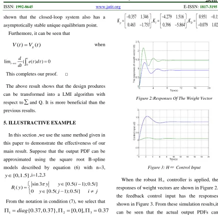
Figure 2:Responses Of The Weight Vector

Figure 3: H∞ Control Input

When the robust H∞ controller is applied, the responses of weight vectors are shown in Figure 2. the feedback control input has the responses shown in Figure 3. From these simulation results,it can be seen that the actual output PDFs can approach its target PDF accurately, it is demonstrated that satisfactory tracking performance,stability and robustness are achieved.

6. CONCLUSIONS

(11)

tracking performance, system stability can be obtained and robustness are guaranteed. A study of an example problem are given to show the efficiency of the proposed algorithms.

REFERENCES:

[l] K.J.Astrom.:Introduction to stochastic control theory. Academic Press, New York, 1970. [2] A.Bagchi.:Optimal Control of stochastic

systems. Prentice Hall international, UK, 1993

[3] Wang Hong.:Bounded dynamic stochastic systems. Springer, London, 2000.

[4] G.A.Smook.:Handbook for Pulp and Paper Technology. AngusWilde Publication Inc., Vancouver, 1992.

[5] H.S.Cho, J.S.Chung, and W.Y.Lee.:Control of Molecular Weight Distribution for Polyethylene Catalyzed over ZieglerNatta/Metallocene Hybrid and Mixed

Catalysts. Journal of Molecular Catalysis A:Chemical, Vol.159(no.2):pp. 203–213, 2000.

[6] T.J.Crowley,K.Y.Choi.:Experimental studies on optimal molecular weight distribution control in a batch-free radical polymerization process. Chemical Engineering Science, Vol. 53(no. 15):pp. 2769–2790, 1998.

[7] F.J.Doyle(III),C.A.Hartison, and T.J.Crowley.:Hybrid model-based approach to batch-to-batch control of particle size

distribution in emulsion

polymerization.Computers & Chemical Engineering,Vol. 27(no. 8 ,9):pp. 1153–1163, 2003.

[8] C.D.Immanuel and F.J.Doyle III.:Open-loop control of particle size distribution in semi-batch emulsion copolymerization using a genetic algorithm. Chemical Engineering

Science, Vol. 57(no. 20):pp. 4415–4427, 2002. [9] Guo Lei,Wang Hong.:Minimum entropy

ﬁltering for multivariate stochastic systems with non-Gaussian noises. In Proc of the ACC. 2005; 315-20.

[10] Guo Lei,Wang Hong.:Fault detection and diagnosis for general stochastic systems using B-spline expansions and nonlinear ﬁlters. IEEE Trans Circuits Syst I.2005; 52(8): 1644-52.

[11] Guo L,Wang H. Entropy optimization ﬁltering for fault isolation of non-Gaussian systems. In Proc of 6th IFAC symposium on fault detection, super-vision and safety of technical processes. 2006; 432-7.

[12] Guo Lei,Wang Hong,Wang.:Optimal probability density function control for NARMAX stochastic systems. Automatica. 2008; 44: 1904-11

[13] Wang Hong,Wang AP,Wang Y.:An online estimation algorithm for the unknown probability density functions of random parameters in stochastic ARMAX systems. IEE Control Theory Applic D. 2006; 153: 462-8.

[14] Guo Lei, Wang Hong. PID controller design for output PDFs of stochastic systems using linear matrix inequalities. IEEE Trans Syst, Man Cybern B 2005; 35(1):65-71.

[15] Yi Yang, Shen Hong, Guo Lei.:Constrained PID tracking control for output PDFs of non-gaussian stochastic based on LMIs.