ISSN: 1992-8645 www.jatit.org E-ISSN: 1817-3195
ENERGY-AWARE NODE PLACEMENT IN WIRELESS
SENSOR NETWORK USING ACO
RABINDRA KU JENA
Institute of Management Technology, Nagpur, India Email: [email protected]
ABSTRACT
The recent popularity of applications based on wireless sensor networks (WSN) provides a strong motivation for pursuing research in different dimension of WSN. Node placement is an important task in wireless sensor network and is a multi-objective combinatorial problem. A multi-objective ACO (Ant Colony Optimization) algorithm based framework has been proposed in this paper. The framework optimizes the operational modes of the sensor nodes along with clustering schemes and transmission signal strengths.
Keywords: Network Configuration, Sensor Placement, Wireless Sensor Networks, ACO.
1. INTRODUCTION
Smart environments represent one of the key future development steps in building, utilities, industrial, home, shipboard, and transportation systems automation. The smart environment basically relies first and foremost on sensory data from the real world. The information needed by smart environments is provided by Distributed Wireless Sensor Networks (DWSN), which are. Wireless sensor networks [1] are composed of a great number of sensor nodes densely deployed in a fashion that may revolutionize information collecting, which makes it a very promising technique for surveillance in military, environmental monitoring, target tracking in hostile circumstances, and traffic monitoring. A wireless sensor network (WSN) is a computer network consisting of spatially distributed autonomous devices using sensors to cooperatively monitor physical or environmental conditions, such as temperature, sound, vibration, pressure, motion or pollutants, at different locations. The development of wireless sensor networks was originally motivated by military applications such as battlefield surveillance. However, wireless sensor networks are now used in many civilian application areas, including environment and habitat monitoring, healthcare applications, home automation, and traffic control.
In addition to one or more sensors, each node in a sensor network is typically equipped with a radio transceiver or other wireless communications device, a small microcontroller, and an energy source, usually a battery. The size a single sensor node can vary from shoebox-sized nodes down to devices the size of grain of dust.[1] The cost of sensor nodes is similarly variable, ranging from hundreds of dollars to a few cents, depending on the size of the sensor network and the complexity required of individual sensor nodes [1]. Size and cost constraints on sensor nodes result in corresponding constraints on resources such as energy, memory, computational speed and bandwidth [1].
with such a high power that their resources could be quickly depleted. Therefore, the collaboration of nodes to ensure that distant nodes communicate with the sink is a requirement. In this way, messages are propagated by intermediate nodes so that a route with multiple links or hops to the sink is established. This paper focuses on these applications, for which it proposes a multi-objective ACO based placement node placement methodology. There are number of reasons that ACO algorithms are a good fit for WSN placement problem.ACO algorithms are decentralized just as WSNs are similarly decentralized. WSNs are more dynamic network, where. nodes can break, run out of energy, have the radio propagation characteristics change. But ACO algorithms have been shown to react quickly to changes in the network.
The rest of this paper is structured as follows. The review of the literature is followed in Section 2, The proposed methodology is formulated in Section 3. Section 4 discusses the multi-objective optimization using ACO. Section 5 discusses the experimental results of the proposed methodology. Finally, conclusions are given in Section 6.
2. RELATED WORK
Extensive wireless sensor network research has focused on almost every layer of the network protocol, including network performance study [2], energy-efficient media access control (MAC) [3], topology control [4] and min-energy routing [5], enhanced TCP [6], and domain-specific application design [7]. Sensor networks are different from other networks due to the limitations on battery power, node densities, and the significant amount of desired data information. Sensor nodes tend to use energy-constrained small batteries for energy supply. Therefore, power consumption is a vital concern in prolonging the lifetime of a network operation. Many applications, such as seismic activity tracking and traffic monitoring, expect the network to operate for a long period of time, e.g., on the order of a few years. The lifetime of a wireless sensor network could be affected by many factors, such as topology management, energy efficient MAC design, power-aware routing, and energy-favored flow control and error control schemes. Different methods for reducing energy consumption in wireless sensor networks have been explored in the literature.
Some approaches [8] were suggested, such as increasing the density of sensor nodes to reduce transmission range, reducing standby power consumption via suitable protocol design, and advanced hardware implementation methodology. Algorithms for finding minimum energy disjoint paths in an all-wireless network were developed [5]. SEAD [9] was proposed to minimize energy consumption in both building the dissemination tree and disseminating data to sink nodes. Few researches have, however, studied how the placement of sensor/aggregation nodes can affect the performance of wireless sensor networks.
On the other hand several interesting approaches like Neural Networks, Artificial Intelligence, Swarm Optimization, and Ant Colony Optimization have been implemented to tackle such problems. Ant Colony Optimization is one of the most powerful heuristics for solving optimization problems that is based on natural selection, the process that drives biological evolution. Several researchers have successfully implemented evolutionary algorithm based techniques i.e Gas, EA, GP etc in a sensor network design [10-13], this led to the development of several other evolutionary based application-specific approaches in WSN design, mostly by the construction of a single fitness function. However, these approaches either cover limited network characteristics or fail to incorporate several application specific requirements into the performance measure of the heuristic. This work tried to integrate network characteristics and application specific requirements in the performance measure of the proposed optimization algorithm based methodology. The algorithm primarily finds the operational modes of the nodes in order to meet the application specific requirements along with minimization of energy consumption by the network. The implementation of the proposed methodology results in an optimal design scheme, which specifies the operation mode for each sensor.
3. PROPOSED METHODOLOGY
ISSN: 1992-8645 www.jatit.org E-ISSN: 1817-3195
control. For monitoring of hypothetical parameters, it is assumed that spatial variability
xρ ϵ X , yρ ϵ Y, zρ ϵ Z are such that xρ << yρ << zρ . It means that the variation of X in the 2D
field is much less than Y and the variation Y is much less than Z. i.e. the density of sensor nodes monitoring Z has to be more than Y and density of sensor nodes monitoring Y has to be more than X in order to optimally monitor the field. The methodology not only takes the general network characteristics into account, but also the above described application specific characteristics.
3.1. Network Architecture Model
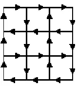
Consider a square field of N x N Euclidian units subdivided into grids separated by a predefined Euclidian distance. The sensing nodes are placed at the intersections of these grids so that the entire area of interest is covered (See Figure 1).
Figure 1. A Grid (Mesh) Based Wireless Sensor Network Layout.
The nodes are capable of selecting one of the three operating modes i.e. X sense, Y sense and Z sense provided they are active. The nodes operating in X sensing mode has the highest transmission range whereas nodes in Y and Z sensing modes have medium and low transmission ranges respectively. Although several cluster based sophisticated methodologies have been proposed [14-16], we have adopted simple mesh architecture, wherein the nodes operating in X sense mode act as cluster-in-charge and are able to communicate with the base station (sink) via multi-hop communication and the clusters are formed based on the vicinity of sensors to the cluster-in-charge. The cluster-in-charge performs tasks such as data collection and aggregation at periodic intervals including some computations. So, X sense node will consume more power than the other two modes.
3.2. Problem Formulation
Here we explore a multi-objective algorithm for WSN design space exploration. The algorithm mainly optimizes application specific parameters, connectivity parameters and energy parameters. This fitness function gives the quality measure of each WSN topology and further optimizes it to best topology. WSN design parameters can be broadly classified into three categories [17]. The first category colligates parameters regarding sensor deployment specifically, uniformity and coverage of sensing and measuring points respectively. The second category colligates the connectivity parameters such as number of cluster-in-charge and the guarantee that no node remains unconnected. The third category colligates the energy related parameters such as the operational energy consumption depending on the types of active sensors. The design optimization is achieved by minimizing constraints such as, operational energy, number of unconnected sensors and number of overlapping cluster- in-charge ranges. Whereas the parameters such as, field coverage and number of sensors per cluster-in-charge are to be maximized. i.e
𝑴𝒊𝒏𝑓( FC, OCE, SOE, SPC ,𝐸) (1)
Where
FC is a field coverage and defined as
𝐹𝐶=(𝑛𝑥+𝑛𝑦+𝑛𝑧)−(𝑛𝑂𝑅+𝑛𝑖𝑛𝑡𝑣)
𝑛𝑡𝑜𝑡 (2)
𝑛𝑥 ,𝑛𝑦𝑎𝑛𝑑 𝑛𝑧 are number of sensors in the
cluster , where 𝑛𝑥 is the cluster in charge.
𝑛𝑂𝑅 is the number of out range sensors, 𝑛𝑖𝑛𝑡𝑣 is
the inactive sensors and 𝑛𝑡𝑜𝑡 is the total sensing point.
OCE is an overlap per cluster in charge error and defined as
𝑂𝐶𝐸=𝑁𝑜_𝑜𝑓_𝑛𝑂𝑣𝑒𝑟𝑙𝑎𝑝𝑠
𝑥 (3)
SOE is the sensor out of range error and is defined as
𝑆𝑜𝐸= 𝑛𝑂𝑅
𝑛𝑡𝑜𝑡−𝑛𝑖𝑛𝑡𝑣 (4)
[image:3.612.152.231.347.436.2]𝑆𝑃𝐶= 𝑛𝑦+𝑛𝑧−𝑛𝑂𝑅
𝑛𝐶 (5)
𝑛𝐶𝑖𝑠𝑡ℎ𝑒𝑛𝑢𝑚𝑏𝑒𝑟𝑐𝑙𝑢𝑠𝑡𝑒𝑟𝑖𝑛𝑐ℎ𝑎𝑟𝑔𝑒
E is the energy consumption and is defined as
𝐸=4.𝑛𝑥+2.𝑛𝑦+𝑛𝑧
𝑛𝑡𝑜𝑡 (6)
4. MULTI-OBJECTIVE OPTIMIZATION
In multi-objective optimization (MO), there are several objectives to be optimized. Thus, there are several solutions which are not comparable, usually referred to as Pareto-optimal solutions. A multi-objective minimization problem with n variables and m objectives can be formulated, without loss of generality, as
𝑚𝑖𝑛𝑦=𝑓(𝑥̅) = min (𝑓1(𝑥̅),𝑓2(𝑥̅), … . ,𝑓𝑚(𝑥̅))
(7)
Where 𝑥̅= (𝑥1,𝑥2… . ,𝑥𝑛) and 𝑦=
(𝑦1,𝑦2… ,𝑦𝑚)
In most cases, the objective functions are in conflicts, so that is not possible to reduce any of the objective functions without increasing at least one of the other objective functions. This is known as the concept of pareto-optimality.
Definition 1 (Pareto Optimal): A point 𝑥̅∈ X is
Pareto optimal if for every 𝑥̅∗∈ X and
I = {1, ..., m} either ∀i∈I, 𝑓𝑖(𝑥̅) = 𝑓𝑖(𝑥̅∗) or,
there is at least one i ∈ I such that 𝑓𝑖(𝑥̅) >𝑓𝑖(𝑥̅∗)
In other words, this definition means that 𝑥̅∗ is Pareto optimal if there exists no feasible vector 𝑥̅ that decrease some criterion without increment in at least one other criterion.
Definition 2 (Pareto Dominance): A vector
𝑢�= (𝑢1,𝑢2… . ,𝑢𝑚) is said to dominate
𝑣̅= (𝑣1,𝑣2… . ,𝑣𝑚) (denoted by 𝑢� ⋞ 𝑣̅ ) if
and only if 𝑢� is partially less that 𝑣̅, i.e., ∀i ∈ {1, . . .,m}, 𝑢𝑖 ⋜ 𝑣𝑖∧∃𝑖∈ {1, . . ., m} : 𝑢𝑖< 𝑣𝑖
A solution α is said to be non-dominated regarding a set 𝑋𝚤 ⊆ 𝑋 if and only if, there is no solution in 𝑋𝚤, which dominates α. The solution α is Pareto-optimal if and only if α is dominated regarding X. The set of all non-dominated solutions constitutes the Pareto optimal set. Therefore, our goal is to find the best Pareto front and near to Pareto optimal.
In order to deal with the multi-objective nature of sensor placement problem we have used multi-objective PSO in our framework.
4.1 ACO Framework
In many real-life optimization problems there are several objectives to optimize. For such multi-objective problems, there is not usually a single best solution but a set of solutions that are superior to others when considering all objectives. This set is called the Pareto set or non dominated solutions. This multiplicity of solutions is explained by the fact that objectives are generally conflicting ones. Recently, different researchers have introduced ACO algorithms for multi-objective problems. These algorithms mainly differ with respect to the three following points. Pheromone trails. The quantity of pheromone laying on a component represents the past experience of the colony with respect to choosing this component. When there is only one objective function, this past experience is defined with respect to this objective. However, when there are several objectives, one may consider two different strategies. A first strategy is to consider a single pheromone structure, as proposed in [18,19]. In this case, the quantity of pheromone laid by ants is defined with respect to an aggregation of the different objectives. A second strategy is to consider several pheromone structures, as proposed in [20,21]. In this case, one usually associates a different colony of ants with each different objective, each colony having its own pheromone structure.
In this section, we present m-ACO a generic ACO framework for multi-objective problems developed by Ines Alay et al [22]. m-ACO is parameterized by the number of pheromone structures #𝜏 Figure 1 describes the generic framework of m-ACO( #𝜏 ). Basically, the algorithm follows the MAX-MIN Ant System scheme [23]. First, pheromone trails are initialized to a given upper bound𝜏𝑚𝑎𝑥. Then, at each cycle every ant constructs a solution, and pheromone trails are updated. To prevent premature convergence, pheromone trails are bounded within two given bounds 𝜏𝑚𝑖𝑛 and
𝜏𝑚𝑎𝑥 such that 0 < 𝜏𝑚𝑖𝑛 < 𝜏𝑚𝑎𝑥. The algorithm
ISSN: 1992-8645 www.jatit.org E-ISSN: 1817-3195
Algorithm m-ACO (#τ)
Initial all pheromone trails to 𝜏𝑚𝑎𝑥 repeat
for each ant k in 1….. #Ants Construct a solution for i in 1….#τ
update the 𝑖𝑡ℎ pheromone structure trails if a trail is lower than 𝜏𝑚𝑖𝑛 then set it to
𝜏𝑚𝑖𝑛
if a trail is greater then 𝜏𝑚𝑎𝑥 then set it to
𝜏𝑚𝑎𝑥
until maximal number of cycles reached
Here #τ is represents the number of objectives.
Algorithm Solution Construction S
S ← Ɵ
Cand ← V
While Cand ≠ Ɵ do
Choose 𝑣𝑖𝜖𝐶𝑎𝑛𝑑 with probability 𝑝𝑆(𝑣𝑖) Add 𝑣𝑖 at the end of S
Remove from Cand vertices that violate constraints
end while
the algorithm used by ants to construct solutions in a construction graph G = (V, E) the definition of which depends on the problem to solve. At each iteration, a vertex of G is chosen within a set of candidate vertices Cand; it is added to the solution S and the set of candidate vertices is updated by removing vertices that violate constraints of C. The vertex 𝑣𝑖 to be added to the solution S by ants of the colony c is randomly chosen with the probability 𝑝𝑆𝐶(𝑣𝑖) defined as follows:
𝑝𝑆𝐶(𝑣𝑖) = [𝜏𝑆
𝐶(𝑣
𝑖)]𝛼 .[𝜂𝑆𝐶(𝑣𝑖)]𝛽
∑𝑣𝑗𝜖𝐶𝑎𝑛𝑑 [𝜏𝑆𝐶(𝑣𝑖)]𝛼 .[𝜂𝑆𝐶(𝑣𝑖)]𝛽 (7)
where 𝜏𝑆𝐶(𝑣𝑖) and 𝜂𝑆𝐶(𝑣𝑖) respectively are the pheromone and the heuristic factors of the candidate vertex 𝑣𝑖. 𝛼 and 𝛽 are two parameters that determine their relative importance. The definition of these two factors depends on the problem to be solved and on the parameter #τ.
The important factors in the above algorithm m-ACO are discussed below:
Pheromone factor: At each step of a solution construction, ants randomly choose an objective r ϵ {1, ...,m} to optimize. The pheromone factor
𝜏𝑆(𝑣𝑗) is defined as the pheromone factor
associated with the randomly chosen objective r.
Heuristic factor: The heuristic factor 𝜂𝑆(𝑣𝑗) considered by the single colony is the sum of heuristic information associated with all objectives,
Pheromone update: Once the colony has computed a set of solutions, the m best solutions with respect to the m different objectives are used to reward them pheromone structures. Let
𝑆𝑖 be the solution of the colony that minimizes
the 𝑖𝑡ℎ objective 𝑓𝑖 for the current cycle, and let
𝑆𝑏𝑒𝑠𝑡𝑖 be the solution that minimizes 𝑓𝑖 over all
solutions built by ants since the beginning of the run (including the current cycle). The quantity of pheromone deposited on a solution component c for the 𝑖𝑡ℎ pheromone structure is defined by
Δ𝜏𝑖(𝑐)
= � 1 (1 +⁄ 𝑓𝑖(𝑆
𝑖)− 𝑓
𝑖(𝑆𝑏𝑒𝑠𝑡𝑖 )) ,𝑖𝑓𝑐𝑖𝑠𝑎
𝑐𝑜𝑚𝑝𝑜𝑛𝑒𝑛𝑡𝑜𝑓𝑆𝑖
0 , 𝑜𝑡ℎ𝑒𝑟𝑤𝑖𝑠𝑒
(9)
5. EXPERIMENTAL RESULTS
ACO involves exploration and tuning of a number of problem specific parameters for optimizing its performance, namely
𝛼,𝛽,𝜌, #𝐴𝑛𝑡𝑠and number of cycles(#cycles) etc. The Table-1 summarized the parameter values considered for the experiment.
Table-1: Parameter Values
𝛼 𝛽 𝜌 #Ants #Cycles
1 4 0.01 100 3000
Figure 2: Final Placement Of Nodes Obtained By M-ACO Algorithm
Figure 3: Performance Of M-Aco Algorithm
6. CONCLUSION
In this paper the node placement methodology for a wireless sensor network using m-ACO based multi-objective methodology is demonstrated. A fixed wireless network of sensors of different operating modes was considered for a 2D grid based deployment. m-ACO algorithm decided which sensors should be active, which ones should operate as cluster-in-charge and whether each of the remaining active normal nodes should have medium or low transmission range. The network layout design was optimized by considering various parameters like application specific parameter, connectivity parameters and energy related parameters. From
the evolution of network characteristics during the optimization process, it concluded that it is preferable to operate a relatively high number of sensors and achieve lower energy consumption for communication purposes than having less active sensors with consequently larger energy consumption.
7. REFERENCES
[1] G. J. Pottie, “Wireless sensor networks,”
Information Theory Workshop 1998, 139-140.
[2] M. Kodialam, T. Nandagopal, “Characterizing the achievable rates in multihop wireless networks,” Mobicom
2003.
[3] T. Dam, K. Langendoen, “An adaptive energy-efficient MAC protocol for Wireless Sensor Networks,” Sensys, 2003 [4] J. Pan, T. Hou, L. Cai, Y. Shi, S. Shen,
“Topology control for Wireless Sensor Networks,” Mobicom, 2003
[5] A. Srinivas, E. Modiano, “Minimum energy disjoint path routing in wireless ad-hoc networks,” Mobicom, 2003
[6] K. Sundaresan, V. Anantharaman, H. Hsieh, R. Sivakumar, “ATP: a reliable transport protocol for ad-hoc networks,” Mobihoc, 2003.
[7] W. Heinzelman, “Application-specific protocol architecture for wireless networks,” Ph.D. Thesis, MIT, 2000.
[8] J. Rabaey, J. Ammer, T. Karalar, S. Li, et al, “Pico-radios for wireless sensor networks: the next challenge in ultra-low power design,” Digest of Technical Papers. ISSCC. IEEE International. Volume 2. 2002 156-445
[9] H. Kim, T. Abdelzaher, W. Kwon, “Minimum-energy asynchronous dissemination to mobile sinks in Wireless
Sensor Network,” Sensys 2003.
[10] R. Min, A. Chandrakasan, “Energy-efficient communication for ad-hoc wireless sensor networks,” Conference Record of the Thirty-Fifth Asilomar Conference on Signals, Systems and Computers. Volume 1. (2001) 139-143.
[11] S. Sen, S. Narasimhan, K. Deb, “Sensor network design of linear processes using genetic algorithms”, Comput. Chem. Eng. 22 (3) (1998), pp. 385–390.
0 5 10 15 20 25
500 1500 3000
Op
tima
l
V
a
lu
es
Cycles
ISSN: 1992-8645 www.jatit.org E-ISSN: 1817-3195
[12] S.A. Aldosari, J.M.F. Moura, “Fusion in sensor networks with communication constraints”, in: Information Processing in Sensor Networks (IPSN’04), Berkeley, CA, April 2004.
[13] R.K.Jena, Multi-Objective Node Placement Methodology for Wireless Sensor Network, International Journal of Computer Applications, IJCA Special Issue on MANETs (2), 2010, p.84–88. [14] O. Younis, S. Fahmy, “Distributed
clustering in ad-hoc sensor networks: a hybrid, energy-efficient approach”, in: INFOCOM 2004, Hong Kong,March, 2004.
[15] M. Younis, M. Youssef, K. Arisha, “Energy-aware routing in cluster based sensor networks”, in: 10th IEEE/ACM International Symposium on Modeling, Analysis and Simulation of Computer and Telecommunication Systems (MASCOTS 2002), Fort Worth, TX, October 2002. [16] S. Bandyopadhyay, E.J. Coyle, “An energy
efficient hierarchical clustering algorithm for wireless sensor networks”, in: IEEE INFOCOM 2003, San Francisco, CA, April 2003.
[17] Konstantinos P. Ferentinos, Theodore A. Tsiligiridis, “Adaptive design optimization of wireless sensor networks using genetic algorithms”, Computer Networks 51 (2007),pp. 1031–1051. [18] B. Baran, M. Schaerer, A Multio bjective
Ant Colony System for Vehicle Routing Problem with TimeWindows, Proc. Twenty first IASTED International Conference on Applied Informatics, Insbruck, Austria, 2003, p. 97-102.
[19] M. Gravel, W. L. Price, C. Gagn´e, Scheduling Continuous Casting of Aluminium using a Multiple Objective Ant Colony Optimization Metaheuristic, European Journal of Operational Research, vol. 143, n1, 2002, p. 218-229. [20] K. Doerner, R. F. Hartl, M. Teimann, Are
COMPETants More Competent for Problem Solving? The Case of Full Truckload Transportation, Central European Journal of Operations Research, vol. 11, No.2, 2003, p. 115-141.
[21] K. Doerner, W. J. Gutjahr, R. F. Hartl, C. Strauss, C. Stummer, Pareto Ant Colony Optimization: A Metaheuristic Approach to Multiobjective Portfolio Selection, Annals of Operations Research, 2004. [22] I. Alaya, Christine Solnon, Khaled
Ghedira, Ant Colony Optimization for Multi-Objective Optimization Problems, ICTAI '07 Proceedings of the 19th IEEE International Conference on Tools with Artificial Intelligence, Vol. 01, 2007, p. 450-457.