ISSN: 1992-8645 www.jatit.org E-ISSN: 1817-3195
A DECISION SUPPORT SYSTEM FOR PREDICTION OF
THYROID DISEASE - A COMPARISON OF MULTILAYER
PERCEPTRON NEURAL NETWORK AND RADIAL BASIS
FUNCTION NEURAL NETWORK
1 SHAIK.RAZIA,2 M.R.NARASINGARAO,3 G R SRIDHAR
1
Research Scholar, Department Of CSE, K L University, Greenfields, Vaddeswaram 2
Professor, Department Of CSE, K L University, Greenfields, Vaddeswaram
3
Endocrine and Diabetes Center, 15-12-16, Krishna Nagar, Visakhapatnam
E-mail: [email protected], [email protected], [email protected]
ABSTRACT
Thyroid disease is a major cause of concern in medical diagnosis and the prediction / onset of which is a difficult proposition in medical research. In this research, we use two Neural Network models Multilayer perceptron (MLP) and Radial Basis Function Networks (RBF) for the prediction of onset of thyroid disease using the data generated in real life. The MLP is trained and tested with Back-propagation algorithm whereas RBF networks was trained and tested with SPSS software. Thyroid disease database which had been published and was used for empirical comparisons and the results show that MLP and RBF show the almost same kind of results in diagnosing the thyroid disease.
Keywords:Neural networks, Radialbasisfunction Network, Multilayer Perceptron, Thyroid Disease, Back-Propagation, Medical Diagnosis.
1. INTRODUCTION
The thyroid is a gland in the neck that produces the hormones that help regulate many body processes, including growth, energy balance, body temperature, and heart rate [1]. The thyroid gland is located at the lower front of the neck. Thyroid function involves the interaction of many hormones, including triodothyronine (T3) and thyroxine (T4). Both of these hormones exist in two forms in the blood and this research can help diagnose hyperthyroidism (when the thyroid gland produces too much thyroid hormone) and hypothyroidism [2] (when the thyroid gland isn't producing enough thyroid hormone). A thyroid stimulating hormone (TSH) test is a common blood test used to evaluate how well the thyroid gland is working. TSH is produced by the pituitary, a pea-sized gland located at the base of the brain. The defects of thyroid function are one production of too little thyroid hormone (hypothyroidism) and second one is production of too much thyroid hormone (hyperthyroidism). In this proposed research, we try to compare two neural network models one is an Multilayer Perceptron Neural Network with sigmoidal activation function and the other is a Radialbasis function network with Gaussian function as the activation function.
1.1 Related Work
ISSN: 1992-8645 www.jatit.org E-ISSN: 1817-3195 Saiti et al in 2009, has proposed SVM and
probabilistic Neural Network as classifier for diagnosing the disease[12]. Rohani et al compared several ANN models for diagnosing the thyroid disease [13]. Eystratios et al proposed an USG image analysis technique for boundary detection of thyroid nodule [14].
1.2 Dataset Description/Thyroid Data Set
The dataset of thyroid gland database taken from the UCI machine learning repository was used as one of the benchmark datasets for testing classifiers. The thyroid data set consists of 215 instances and each instance has five attributes plus the class attribute. All samples have five features. We used attributes of the thyroid disease along with network parameter bias were considered as a set of inputs and assessed the performance of the networks in predicting the thyroid disease. Three scales of measurement was considered as outputs of the network in this research and they were considered as Normal, Hypothyroidism and Hyperthyroidism respectively [15]. The inputs and outputs were taken as follows.
• T3: Resin uptake test
• Total serum thyroxin as measured by the isotopic displacement method
• Total serum triodothyronine as measured by radio immuno assay
• Basal thyroid stimulating harmone (TSH) as measured by radio immune assay
• Maximal absolute difference of TSH value after injection of 200micro grams of thyrotropin-releasing hormone as compared to the basal value
• Class attribute in which 1 for Normal, 2 for hyperthyroid and 3 for Hypothyroid were taken as outputs.
All attributes are continuous and each of the instances has to be categorized into one of the three classes. Class-1: Normal (150 instances) Class-2 Hyperthyroidism (35 instances) and Class-3: Hypothyroidism (30 instances).
The table-1below describes the class distribution of each type of disease
Type of disease Number of samples class
Normal 150 1
Hyperthyroidism 35 2 Hypothyroidism 30 3
Total 215
2. MULTILAYER PERCEPTRON NEURAL NETWORKS
Artificial Neural Networks is an important application of Artificial Intelligence and is an attempt to model the functioning of the human brain. Single Layer Perceptrons (SLP) are those that have only one input and one output layer. SLP’s are normally used in developing filters. Input layer is a layer which consists of input neurons and output layer is a layer consists of output neurons. Input layer is responsible for taking the inputs and output layer is responsible for generating the outputs. Neural Networks provide a mapping between input neurons in the input layer and output neurons in the output layer. This mapping provided by the network varies with the data set used for the network. An inbuilt function will be developed internally by the network. The connection between Neurons in the input layer and the neurons in the output layer are called as synapses and each synapse is associated with a weight called as a synaptic weight. Multi Layer Perceptron is a feed-forward neural network with one or more number of hidden layers between input and output layer. Feed-forward networks are those networks where the information flows from input to output layer in a forward direction. This network is trained with the supervised learning algorithm called as a back-propagation learning algorithm and classified the data into 3 subclasses. The back propagation algorithm is as follows.
2.1 After presenting input data to the input layer, information propagates through the network to the output layer (forward propagation). During this time, input and output states for each neuron will be set.
ISSN: 1992-8645 www.jatit.org E-ISSN: 1817-3195 Where
Xj [s] - Denotes the current input state of the jth neuron in the current [s] layer.
Ij [s] - Denotes the weighted sum of inputs to the jth neuron in the current layer[s].
f is conventionally the sigmoid function.
wij[s] - denotes the connection weight between the I th neuron in the current layer [s] and j th neuron in the previous layer [s-1]. [16]
2.2 Global error is generated based on the summed difference of required and calculated output values of each neuron in the output layer. The Normalized System error E (glob) is given by the equation [16]
E(glob)= 0.5 * (rk - ok)2
and (rk - ok) denotes the difference of required and calculated output values.
2.3 Global error is back propagated through the network to calculate local error values and delta weights for each neuron. Delta weights are modified according to the delta rule that strictly controls the continuous decrease of synaptic strength of those neurons that are mainly responsible for the global error. In this manner the regular decrease of global error can be assured. [16]
Ej[s]=Xj[s] * (1.0-xj[s])*∑(ek[s+1] * wkj[s+1]) Where
Ej[s] = Scaled local error of the jth Neuron in the current layer [s]
Δwji[s]=lcoef * ej[s]*xi[s-1]
Δwji[s] = Denotes the delta weight of the connection between the current neuron and joining neuron. lcoef denotes the learning co-efficient / learning constant of the training parameters[16]
2.4 Synaptic weights are updated by adding delta weights to the current weights
3. RADIAL BASIS FUNCTION NETWORKS
In this article an attempt is made to study the applicability of a general purpose, supervised feed forward neural network with one hidden layer, namely, Radial Basis Function (RBF) neural network. It uses relatively smaller number of locally tuned units and is adaptive in nature. It is an artificial neural networks that uses radial basis functions as activation functions. The output of a network is a linear combination of radial basis functions of the inputs and neuron parameters. These type of networks are used in classification, function approximation, time series prediction and
system control. The methodology of Radial Basis Function network is as follows. [17]
The RBF network has a feed forward structure consisting of a single hidden layer of J locally tuned units, which are fully interconnected to an output layer of L linear units. All hidden units simultaneously receive the n-dimensional real valued input vector X (Figure 2). The main difference from that of MLP is the absence of hidden-layer weights. The hidden-unit outputs are not calculated using the weighted-sum mechanism/sigmoid activation; rather each hidden-unit output Zj is obtained by closeness of the input
X to an n-dimensional parameter vector mj associated with the jth hidden unit10,11.The response characteristics of the jth hidden unit ( j = 1, 2, , J) is assumed as,
Zj = K
−
2
j
j
X
σ
µ
--(1)
Where K is a strictly positive radially symmetric function (kernel) with a unique maximum at its ‘centre’ mj and which drops off rapidly to zero away from the centre. The parameter σj is the
width of the receptive field in the input space from unit j. This implies that Zj has an appreciable value only when the distance
X
−
µ
j
is smaller than the width σj. [17]Given an input vector X, the output of the RBF network is the L-dimensional activity vector Y, whose lth component (l = 1, 2 ……., L) is given by,
YƖ (X) =
)
(
1W
Z
jX
J
j lj
∑
=--(2)
For l = 1, mapping of eq. (1) is similar to a polynomial threshold gate. However, in the RBF network, a choice is made to use radially symmetric kernels as ‘hidden units’. RBF networks are best suited for approximating continuous or piecewise continuous real-valued mapping f : Rn -->RL, where n
ISSN: 1992-8645 www.jatit.org E-ISSN: 1817-3195 networks can be controlled by three parameters: the
number of basis functions used, their location and their width. In the present work we have assumed a Gaussian basis function for the hidden units given as Zjfor j = 1, 2, ….., J where
−
−
=
22
exp
j j
j
X
Z
σ
µ
-(3)
and µjand σjare mean and the standard deviation
respectively, of the j th unit receptive field and the norm is the Euclidean.[17]
A training set is an m labelled pair {Xi, di} that
represents associations of a given mapping or samples of a continuous multivariate function. The sum of squared error criterion function can be considered as an error function E to be minimized over the given training set. That is, to develop a training method that minimizes E by adaptively updating the free parameters of the RBF network. These parameters are the receptive field centres mj
of the hidden layer Gaussian units, the receptive field widths sj, and the output layer weights (wij).
Because of the differentiable nature of the RBF network transfer characteristics, one of the training methods considered here was a fully supervised gradient-descent method over E. In particular, µj,σj
and wijare updated as follows: [17]
∆
µ
j=
−
ρ
µ∇
µ
jE
---(4)
j j
E
σ
ρ
σ
σ∂
∂
−
=
∆
---(5)
lj w ij
w
E
w
∂
∂
−
=
∆
ρ
---(6)where
ρ
µ,
ρ
σ,
and
ρ
w, are small positive constants. This method is capable of matching or exceeding the performance of neural networks with back-propagation algorithm, but gives training comparable with those of sigmoidal type of FFNN.The training of the RBF network is radically different from the classical training of standard FFNNs. In this case, there is no changing of weights with the use of the gradient method aimed at function minimization. In RBF networks with the chosen type of radial basis function, training resolves itself into selecting the centres and dimensions of the functions and calculating the
weights of the output neuron. The centre, distance scale and precise shape of the radial function are parameters of the model, all fixed if it is linear. Selection of the centers can be understood as defining the optimal number of basic functions and choosing the elements of the training set used in the solution. It was done according to the method of forward selection. Heuristic operation on a given defined training set starts from an empty subset of the basis functions. Then the empty subset is filled with succeeding basis functions with their centres marked by the location of elements of the training set; which generally decreases the sum-squared error or the cost function. In this way, a model of the network constructed each time is being completed by the best element. Construction of the network is continued till the criterion demonstrating the quality of the model is fulfilled. The most commonly used method for estimating generalization error is the cross-validation error. [17]
4. RESULTS
4.1 RBF Neural Network
The RBF Neural Network was trained and tested with SPSS software.
The table given below (Table -1) describes percentage of sample taken by the network for classification purpose.
Table-1: The Case Processing Summary Of The Network N Percent Sample Training 152 76.8
Testing 46 23.2
Valid 198 100
Excluded 17
Total 215
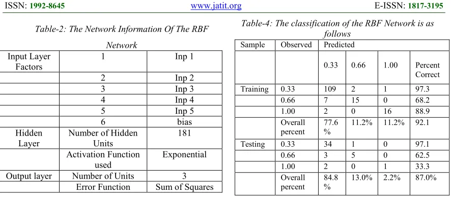
ISSN: 1992-8645 www.jatit.org E-ISSN: 1817-3195 Table-2: The Network Information Of The RBF
Network Input Layer
Factors
1 Inp 1
2 Inp 2
3 Inp 3
4 Inp 4
5 Inp 5
6 bias
Hidden Layer
Number of Hidden Units
181 Activation Function
used
Exponential Output layer Number of Units 3
Error Function Sum of Squares The following table (Table-3) describes the error generated by the network along with percentage of incorrect predictions during testing and training phases of the network.
[image:5.612.86.531.76.270.2]
Table-3: The Model summary of the RBF network is as follows
Training Sum of squares error
10.501 Percent incorrect
predictions
7.9% Testing Sum of squares
error
5.057 Incorrect
predictions
13.0%
The following table (Table-4) gives the entire classification made by the RBF network during training and testing phases. It is observed that RBF network classified the entire dataset into 77.6% as Normal, 11.2% as Hypothyroidism and finally 11.2% as Hyper-thyrodism during training phase.
In testing phase, 84.8% was considered for Normal, 13.0% and 2.2% was considered for Hypothyroidism and Hyperthyroidism individually respectively.
In a nut shell, the RBF network classified 92.1% during training phase and 87% during testing phase respectively.
Table-4: The classification of the RBF Network is as follows
4.2 MLP Neural Network
The MLP Neural Network was developed using back-propagation algorithm. Many Network parameters were considered during training and testing phases of the network. The network parameters considered are number of input samples, number of output samples, learning rate, momentum rate, maximum individual error, maximum total error, number of iterations respectively. The input to the MLP network was taken from a data (.dat) file. Six input neurons including the bias were considered in the input layer and 3 neurons were considered in the output layer respectively. The output generated by the network is predicted by considering the Normalized System Error values of the network. The following table gives the Normalized System Error (NSE) values generated by MLP Neural Network for different input samples and for different neurons in each hidden layer.
Table-5( NSE values of the MLP Network w.r.t input samples and hidden neurons)
Table-5 Placed at the end of paper
The following table (Table-6) gives the accuracy given by the network. Here Input-1 to Input-6 was taken as inputs and the actual value is the value generated by the network during testing phase. It is observed that, 99% accuracy is maintained by the MLP for Normal, 49.5% for Hypothyroidism and finally 33% for Hyperthyroidism for predicting the disease. When compared with RBF, MLP is slightly more accurate in predicting the disease. The testing of the MLP Network is given in the following table.
Table-6:(Accuracy of the MLP Network)
Sample Observed Predicted
0.33
0.66
1.00
Percent Correct
Training 0.33 109 2 1 97.3
0.66 7 15 0 68.2
1.00 2 0 16 88.9
Overall percent
77.6 %
11.2% 11.2% 92.1
Testing 0.33 34 1 0 97.1
0.66 3 5 0 62.5
1.00 2 0 1 33.3
Overall percent
84.8 %
[image:5.612.84.304.354.443.2]ISSN: 1992-8645 www.jatit.org E-ISSN: 1817-3195
Table-6 Placed at the end of paper
Limitations of the work
As any project consists of pros and cons , this proposed research also consists of some limitations.
• Usually the problem given to the neural network is described as a set of examples rather than a function. Therefore the number of points in the problem space is finite. Neural networks which are trained properly have a good interpolation performance, but a very poor extrapolation performance. Unfortunately there is no general rule to find out if a new pattern is within the interpolation space
• The prediction accuracy could be more had we considered more number training and testing samples.
• The system can be enhanced to any desired level if we provide more number of inputs and outputs.
• The proposed system can also be used for different kinds of disease diagnosis given the set of input and output variables.
DISCUSSION:
The Multilayer Perceptron Neural Network has been trained by back propagation algorithm and Radial Basis Function Network has been trained by SPSS software to predict thyroid disease using biological variables. Neural Network models have been employed in a variety of clinical medicine settings, but this is the first time it is being used to predict the onset of thyroid disease [18]. The comparison of two models (MLP & RBF Networks) had been done to predict the onset of thyroid disease. The results indicate that, Normal outcome had been recognized /classified by both the networks accurately whereas which is not the same for Hypothyroidism and Hyperthyroidism labels. This is because; both the networks have not been trained and tested with more number of Hypothyroidism and Hyperthyroidism variables and which is due to lack of values for these
variables in the dataset gathered from UCI library . The development of our model is a practical tool to predict thyroid onset variables and as more data are generated the system improves in precision and can be widely employed in patient care and research.
CONCLUSION
It is seen that radial basis network can be successfully used for the diagnosis of thyroid disease. Diagnosing the thyroid disease is an important yet difficult task from both clinical diagnosis and statistical classification point of view. In summary, in this proposed research, we developed two Neural Network models using the available information on thyroid disease diagnosis demonstrated that it gave results consistent with our recent application of the method to predict wellbeing[16]
REFERENCES:
[1] Rastogi, Astha Bhalla, Monika, A Study of Neural Network in Diagnosis of Thyroid,in International Journal of Computer Technology and Electronics Engineering (IJCTEE) Vol 4, Issue 3, June 2014.
[2] Zhang, Guoqiang Peter Berardi, Victor L, An investigation of neural networks in thyroid function diagnosis In Health Care Management Science,vol.1,issue1,pages29-37 [3] J.Margret ,B. Lakshmipathi and S.A.Kumar , “Diagnosis of Thyroid Disorders using Decision Tree Splitting Rules”,International Journal of Computer Applications (0975 – 8887) Volume 44– No.8, April 2012.
[4] F. S. Gharehchopogh, M. Molany and F. D.Mokri,”USING ARTIFICIAL NEURAL NETWORK IN DIAGNOSIS OF THYROID DISEASE: A CASE STUDY”, International Journal on Computational Sciences & Applications (IJCSA) Vol.3, No.4, August 2013.
[5] S.B Patel , P. K Yadav, Dr. D. P.Shukla,”
ISSN: 1992-8645 www.jatit.org E-ISSN: 1817-3195 [6] Chuan-Yu Chang, Ming-Fang Tsai and Shao-Jer
Chen,“ Classification of the Thyroid Nodules Using Support Vector Machines” International joint conference on Neural Networks 2008, pp 3093- 3098.
[7] D.E. Maroulis, M.A. Savelonas and S.A. Karkanis, “Computer –Aided Thyroid Nodule Detection in Ultrasound Images” 18th IEEE International Symposium on computer based medical systems(CBMS’05),2005.
[8]M. Savelonas, D. Maroulis, D. Iakovidis and S. Karkanis, “Variable Background Active Contour Model for Automatic Detection of Thyroid Nodules in Ultrasound Images “, 2005.
[9] I.S.Isa,Z.Saad,S.Omar,M.K.Osman,K.A.Ahma ,”Suitable MLP Network Activation Functions for Breast Cancer and Thyroid Disease Detection” ,Second international conference on computational intelligence,modelling and simulation,2010 IEEE, pp 39 – 44.
[10] Canon SENOL,Tulay YILDIRIM, “Thyroid and Breast Cancer Disease Diagnosis using Fuzzy-Neural Network “, unpublished. [11] Anupama Shukla,Prabhdeep Kaur, “Diagnosis
of thyroid disorders using artificial neural networks ” ,2009 IEEE International Advance computing Conference(IACC 2009)– Patiala ,India , 2009, pp 1016-1020.
[12] Fatemah Saiti,Afsaneh Alavi Naini,Mahdi Aliyari shoorehdeli,Mohammad Teshnehlab, “Thyroid disease diagnosis based on genetic algorithm using PNN & SVM”, 2009 IEEE, pp 1-4
[13] Modjtaba Rouhani,Kamran Mansouri, “Comparison of several ANN architectures on the thyroid diseases grades diagnosis ” , 2009 International Association of computer science and information technology-spring conference, 2009, pp 526-528.
[14] Eystratios G.Keramidas,Dimitris K.Iakovidis,Dimitris Maroulis and Stavros Karkanis “Efficient and effective image analysis scheme for thyroid nodule detection “.
[15] Dr. Sahni BS, Thyroid Disorders [online].
Available :
http://www.homoeopathyclinic.com/articles/d iseases/thyroid.pdf
[16] NarasingaRao MR,Padmaja, TM Sridhar, GR Lind, Marcus,Madhu, K,Ramakrishna, Assessment of Wellbeing in Diabetes-A Comparison of MLP with Back-propagation and Support Vector Regression, 2013
[17] P.Venkatesan, S.Anitha, “ Application of RBF Neural Network for diagnosis of Diabetes Mellitus”, Current Science, Vol. 91, No. 9, 10 November 2006, 1195-99
ISSN: 1992-8645 www.jatit.org E-ISSN: 1817-3195
Table-5( NSE values of the MLP Network w.r.t input samples and hidden neurons)
Neurons/ 1 2 3 4 5 6 7 8 9 10
Samples
10 0.22449 0.019176 0.017409 0.011186 0.010819 0.009982 0.010983 0.012875 0.009982 0.013624 20 0.016912 0.00995 0.009912 0.009992 0.01 0.009957 0.009998 0.009998 0.009922 0.009967 30 0.015836 0.009992 0.009946 0.009971 0.009942 0.009964 0.009986 0.009994 0.009981 0.009997 40 0.013384 0.009933 0.00995 0.009941 0.009958 0.009946 0.009967 0.009984 0.009993 0.00997 50 0.012126 0.009951 0.00996 0.00997 0.009934 0.009967 0.009964 0.00993 0.009955 0.009981 60 0.011987 0.009877 0.009882 0.00989 0.009897 0.009989 0.009952 0.00993 0.009959 0.009958 70 0.012236 0.009987 0.009849 0.009949 0.009903 0.009948 0.009885 0.00994 0.009964 0.009922 80 0.011356 0.009849 0.009899 0.009905 0.009969 0.009934 0.009884 0.009904 0.009893 0.009913 90 0.01075 0.009853 0.009903 0.009951 0.009851 0.009871 0.009866 0.009906 0.009948 0.009938 100 0.011203 0.009762 0.009752 0.009999 0.009991 0.009837 0.009842 0.009976 0.009999 0.009955 110 0.010339 0.010485 0.009812 0.009929 0.009763 0.00987 0.009937 0.009901 0.009882 0.009872 120 0.010355 0.009828 0.009792 0.009936 0.009835 0.009872 0.009942 0.00998 0.009926 0.009957 130 0.010256 0.009981 0.009869 0.009785 0.00996 0.009884 0.009982 0.009932 0.009843 0.009964 140 0.010706 0.00967 0.009782 0.009901 0.009964 0.00985 0.009875 0.009888 0.009812 0.009859 150 0.011901 0.009558 0.009981 0.009831 0.009897 0.009805 0.009974 0.009889 0.00979 0.009861
Table-6:(Accuracy of the MLP Network)
Input1 Input2 Input3 Input4 Input5 Input6 Actual Value Desired value %of accuracy 1 0.84 0.19 0.18 0.2 0.94 0.98 1 98