7 4 5a Three Mode Controller 1964 pdf

(1)

* Studies included within the EDUCATIONAL classification are, in most cases, derived from the broad spectrum of scientific and engineering

computer applications. Their presentation is oriented toward classroom or laboratory use, and they deal with problems appropriate for chemical, electronics, bio-medical, etc., courses. For the convenience of users in specific industrial fields, however, all EDUCATIONAL studies are cross-referenced in the Applications Library Index under the industrial octivity(ies} with which they are most closely associated.

THREE MODE CONTROLLER

INTRODUCTION

This Study, performed on a PACE0TR-I0

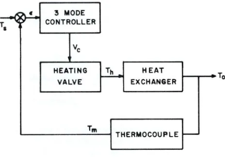
desk-top-size general purpose analog computer, des-cribes an investigation of the operation of a three-mode temperature control system. In the diagram of Figure 1, a three mode controller is used to control the output temperature, To, of a heat

ex-changer. The measured temperature, T m, is

compared to a desired set point temperature, T s, and the difference between these two temperatures results in an error voltage, E. This error VOltage

J'C"C :5 MODE

T. ~?' CONTROLLER

Vc

PROPORTIONAL RESET RATE

"J<" C vp If:' vr j ( Vc

m~?' Kp C 'I; _'9'

To

T.

-

J

r--

' - -

-

d

[image:1.611.318.555.213.338.2] [image:1.611.51.283.385.550.2]

r--dt

Figure 2. Block Diagram of Three Modes

provides the control voltage, V c, with an integral of the error voltage. Its function is to reduce the steady state error signal to zero. The rate section of the controller provides the control voltage with a derivative of the output of the reset section of the controller. Its function is to" antiCipate" tempera-ture Changes and to smooth out transient response

To of the temperature control system.

HEATING

_~

HEAT

EXCHANGER VALVE

Tm

THERMOCOUPLE

-Figure 1. Simplified Diagram of Three Mode Controller Used to Control Temperature

is used by the controller to supply a control voltage, V c, to the heating valve. The heating valve, in turn, controls the input heat, Th, to the eXChanger. Any changes in To are sensed by the thermocouple and fed back to the input of the controller, which is adjusted to provide close control of To during both steady state and transient temperature conditions. A simplified block diagram of the three mode con-troller is shown in Figure 2.

The proportional section of the controller provides straight gain to the error signal. The reset section

1

System Equations

Differential Form

1. Heat Exchanger

. 1 1

T_o+ - T =- T

T O T h

e e

2. Heating Valve

3. Thermocouple

. 1 1

T +- T =- T

m T

t m T

t 0

Transfer Function

T

--2. (S) 1

Th = ~

(2)

4, Controller

A, Proportional

B, Reset

v

+ l

/v

dt=V

p Kr 0 p r

C, Rate

-v 1 + -1

f

(V +V)dt=V

a r aKd r c c

V K S + 1

vr(S)=+S-p r

Range of Parameters and Variables

1. Controller

Kp Proportional Gain 0< Kp ~ 10 Kr Reset Time 00 ~ Kr ~ 1 sec.

Kd Rate Time oo~ Kd ~,1 sec,

ac Compensation Ratio ₌₁₀1

Ts Set Point Temperature 0~Ts~100°

Vp Proportional Voltage

o

~ Vp ~ 10 v Vr Reset Voltage

o

~ Vr ~ 10 v 2. Exchanger

To Output Temperature

o

to 1000 _F

Th Input Temperature

o

to 1000 _F Te Time Constant = 2 sec.

3. Thermocouple

Tm Thermocouple Output

o

to 1000 F Tt Time Constant = 1 sec.

4. Valve

Wn Natural Frequency = ~ radians/sec. Vc Valve Input Voltage

o

to 10 v

~ Damping Factor = .7 C Control Constant = 1 V/10°F

Problem Statement

Develop a computer program to investigate the operation of the control system operating at dif-ferent set points and difdif-ferent values ofproportional gain, reset, and rate, Exchanger output tempera-ture and temperatempera-ture error should be plotted with respect to time,

Develop the following:

a) Scaled Equations

b) Computer Circuit Diagram

c) Amplifier and Attenuator Sheets for the Runs Given Below

d) Static Check

First Run

T = 20° F

s

K =5

P

K = COsec,

r

Kd = ,I sec.

Place the computer in the operate mode and Slowly raise the temperature set point to 20° F, Note the temperature error on the computer voltmeter, Slowly raise the temperature set point to 50° F and again note the temperature error,

Second Run

T = 20° F

s

K =5

P

K = 20 sec,

r

Kd = ,I sec,

Repeat run #1 with the rate time set at 20 seconds,

Third Run

T = 20° F

s

K

=5

p

K = 20 seconds

r

Kd = .1 second

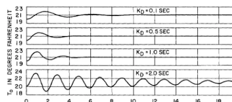
Place the computer in operate and slowly raise T s to 20° F. Allow the system to reach steady state operation and then apply a 1°F step to the temperature set point, Record To with respect to time for each of the following values of Kd:

0,1 sec, 0,5 sec" 1 sec. and 2 sec,

Observe the speed of response of To and the amount of time it takes To to reach the steady state value,

Fourth Run

(3)

step of 10 F. Optimum operation is considered

to be quick response to a step input with little temperature overshoot and a very small static error. The system also should be stable and not tend to oscillate. Record the values of Kp , Kr and

Kct

for what is considered optimumresponse.

Introduction to Solution

The system equations given above are re-written so that the highest order derivative is on the left side of the equal sign. A basic computer diagram is now sketched out to solve the system equations. This diagram is drawn without regard for equation scaling. It is used to find out roughly how much equipment is needed and to gain an understanding of any equation manipulation which might result in a more simplified computer model.

A rough computer program is given in Figure 3. Using this circuit, the followingequipmentcomple-ment will be required:

6 Integrators

4 Summing Amplifiers 3 Inverters

19 Attenuators (6 of which are used for static test Ie's)

Scaled Equations

The first step in obtaining scaled equations is to rewrite the system equations so that the highest derivative appears on the left side of the equation

1. (Exchanger)

2. (Valve)

3. (Thermocouple)

4. ( Proportional)

1

It

B. V = V + - V dt

r p Kr 0 p

(Reset)

1

It

c.

V

=...!..v

+ - - (V -V) dt

c a r aKd 0 r c (Rate)

Next, scale factors are obtained by dividing the reference voltage by the maximum value of the variable.

[image:3.623.79.532.376.685.2]

(4)

Variable Max. Value Scale Factor Computer Variable

T 100" F 10

[to

ToJ

0 100

Th 100" F

10

[to

ThJ 100

V lOV .!Q..

[VcJ

c 10

T 100' F 10

[to

_TmJ

m 100

T 100" F 10

[;0 TsJ

5 100

V 10 V 10

[VpJ

p

10

V 10 V 10

[VrJ

r 10

T 10"/see 10

[ToJ

0

10

T 10" /see 10

[TmJ

m

10

Th lOY/see 10 ₁₀ _[ThJ

The following scaled voltage equations were ob-tained:

1.

~~~J

=

(:J

f:o

Th] -

(;J

[io

To] (Exchanger)

2.

[:~J

= 20

C:!e

)~cJ

-10

e:;~)t~~] -20~:;)~

(Valve)

3. ~=(T:)[ToTo] -(T:)[ToT~

(Thermocouple)

4. -10

fe

K ) [.2.. T _.2.. T

J

=

[V

1

\ p 10 m 10 s PJ ( Proportional)

[v

r] = + [Vp] +

(~r) ~t

Vp

d~

(Reset)

[Vc] = +-;;

[v

r] +-;; [Kd][.( (Vr-Vc) dtJ (Rate)

In the above equations

--The numbers preceding the brackets are ampli-fier gains;

The quantities in the square brackets are com-puter voltages;

The coefficients in the curved brackets are attenuator settings,

PROBLEM MECHANIZATION

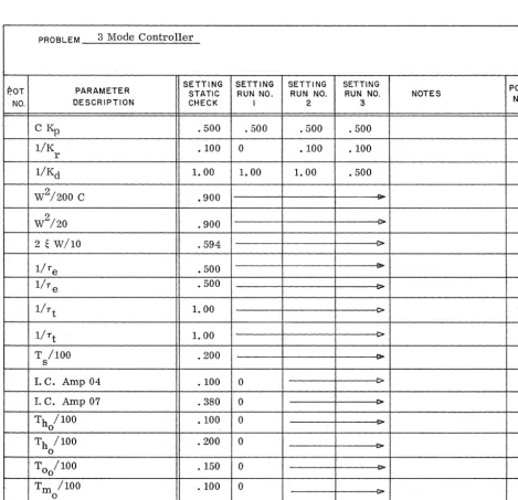
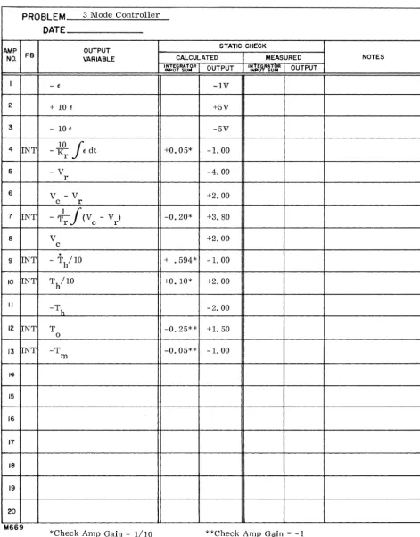
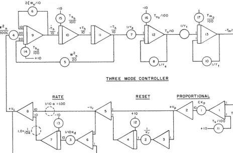
The potentiometer and amplifier assignment sheets are shown in Figures 4 and 5, The scaled com-puter diagram is shown in Figure 6,

Static Check

To check the scaled equations, computer circuit, patching and equipment, a static check is prepared using the original equations.

Let Th T 0 T m T s V c

= 20' F

= IS' F

.

= 10' F

~ 20' F

= 2v

of =

h 10' F/sec.

K

P

Te

T t

e

1 t

Kr

f

Vp dt = -1 V

o

= 5

= 2 sec.

= 1 sec.

= 1 V/I0' F

t

-K1

f

(V + V ) dt = +3. 80 V

d r c

o

Substituting these values into the original equations and solving for the highest derivatives:

T

+.!.x20"=.!.x15"

o 2 2

T =2.5'/sec.

o

w

2 V

2. Th+Wn'2~Th+W!Th=~

., 18.2

Th + 18 • 2 • 0.7 • 10 + 18 • 20 = 1/10 Th = 360 - 59.5 - 360 = -59.5" F/sec/soo.

3. T +.2..T =l.T

m

't

m T_t 0

T + 1 • 10 = 1 • 15

m

T _m= 5" F/sec.

4. Controller

A. K (T - T ) (C) = V

p s m p

5 (20' - 1O")..!.. = V

10 l>

V =5V p

1

it

B. v +j{ V dt = V

P r o p r

5+-1V=V

r

V =4V

r

c.

2. V + - K1

frv

+ V ) dt = V

a r a

dJ'

r c c 10.4 - 10 ' 3. 8 = V

c

(5)

PROBLEM 3 Mode Controller

SETTING SETTING SETTING SETTING _POT

P.OT PARAMETER _STATIC _{RUN NO.} _{RUN NO.} _{RUN NO.} _NOTES

NO.

NO. DESCRIPTION CHECK I 2 3

C Kp, .500 .500 .500 .500

l/K .100 0 .100 .100

r

l/Kd 1. 00 1. 00 1. 00 .500

W2/200 C .900

W2/20 .900

2 ~ W/10 .594 ~

l/Te .500

l/T e .500

l/r

_t

1. 00

l/ T

_t

1. 00 ~

T /100 .200

s

I. C. Amp 04 .100 0

1. C. Amp 07 .380 0

Th /100 .100 0

0

Th /100 .200 0

0

To /100 .150 0

0

Tm /100

0

.100 0

[image:5.627.59.529.111.564.2]

(6)

PROBLEM

3 Mode Controller

DATE

AMP OUTPUT STATIC CHECK

NO. FB VARIABLE CALCULATED MEASURED NOTES

',~~5¥R:J3R OUTPUT I~N1.~G,-Rm: OUTPUT

I

_-

_~ _-IV

2 _{+ 10}_~ _+5V

3 _{- 10}~ -5V

4 _INT _{- Kr}10

f

_~_dt _+0.05* _-1.₀₀

5 - V -4000

r

6 _{V -V} _+2.00

c r

7 INT

- f-j(V -

V ) -0.20* +3.80

r c r

8 V +2.00

c

9 INT - +/10 + .594* -1. 00

10 INT T/10 +0. 10* +2.00

((

-Th -2.00

12 INT T -0.25** +1. 50

0

13 INT -T -0.05** -1. 00

m

14

15

16

17

18

19

20

'-4669

*Check Amp Gain = 1/10 **Check Amp Gain = -1

[image:6.624.68.539.51.652.2]

(7)

HEATING VALVE

2eWn/i0

-10

II

5

EXCHANGER THERMOCOUPLE

-10

T oliO

THREE MODE CONTROLLER

RATE RESET PROPORTIONAL

Figure 6. Scaled Computer Diagram

It should be noted that some of the above values are integrator inputs which cannot be checked di-rectly. The output of an integrator in RESET is simply its initial condition and is independent of the inputs. Therefore, the inputs from the integrator are transferred temporarily to a spare summing amplifier, read, and then patched back into the integrator where they belong. By doing this for each integrator in turn, the values of all the in-tegrator inputs can be verified.

When temporarily transferring inputs from an in-tegrator to a summer, use the actual inin-tegrator input resistors. This insures that both the leads and input resistors are checked. Since a summer with a 10K feedback has 1/10 the gain that an in-tegrator with the same input resistor would have, the output of the amplifier used for checking is 1/10 (TOTAL INPUT TO INTEGRATOR).

Conclusion

When the three mode controller is operated without reset, there will be an error between the set point temperature and the exchanger temperature. The exchanger output temperature will always be lower than the set point temperature.

If reset is added to the temperature control, the error between the set point temperature and the exchanger temperature will eventually be zero. The amount of time that it takes the temperature error to go to zero depends on the reset time. A high value of reset time will result in a long time for the temperature error to reach zero and vice-versa. However, if the reset time is made too short, the system will tend to be unstable.

[image:7.626.74.539.33.338.2]

(8)

faster. The output temperature of the exchanger will rise more quickly to its new value and will reach. steady state operation faster. If too much rate is added, the system will tend to oscillate. A graph of exchanger output temperature versus time for different rate times is given in Figure 7.

In this problem, the temperature set pOints and

temperature s t e p s were purposely kept low in order to operate all of the equipment in its linear range. Although the values used are not realistic, the basic operation of the three mode controller is. After running this problem, one should have a thorough understanding of how a three mode con-troller operates and how it may be simulated on an analog computer.

I KD -0.1 SEC

I I KD -0.5 SEC

I I

o 2 4 6 8 10 12 14 16 18 20 TIME IN SECONDS

Figure 7. Exchanger Output Temperature vs Time

EAI

®

ELECTRONIC ASSOCIATES, INC. Long Branch, New Jersey

[image:8.630.185.423.164.269.2]