A Distributive Approach for Data Collection Using SenCar in Wireless Sensor Networks

(1)

Page 428

A DISTRIBUTIVE APPROACH FOR DATA COLLECTION USING SENCAR IN

WIRELESS SENSOR NETWORKS

A.Mythili

1

_{, T.Prabakaran}

2

1

_{PG Scholar, ECE, SNS College of Technology, Coimbatore, India}

2

_{Associate professor, ECE, SNS College of Technology, Coimbatore, India}

---Abstract -

a three-layer framework is proposed for

mobile data collection in wireless sensor networks, which includes the sensor layer, cluster head layer, and mobile collector (called SenCar) layer. The framework employs distributed load balanced clustering and dual data uploading, which is referred to as LBC-DDU. The objective is to achieve good scalability, long network lifetime and low data collection latency. At the sensor layer, a distributed load balanced clustering (LBC) algorithm is proposed for sensors to self-organize themselves into clusters. In contrast to existing clustering methods, our scheme generates multiple cluster heads in each cluster to balance the work load and facilitate dual data uploading. At the cluster head layer, the inter-cluster transmission range is carefully chosen to guarantee the connectivity among the clusters. Multiple cluster heads within a cluster cooperate with each other to perform energy-saving

inter-cluster communications. Through inter-cluster

transmissions, cluster head information is forwarded to SenCar for its moving trajectory planning. At the mobile collector layer, SenCar is equipped with two antennas, which enables two cluster heads to simultaneously upload data to SenCar in each time by utilizing multi-user

multiple-input and multiple-output (MU-MIMO) technique.

Key Words:

Load balanced clustering algorithm, Data

collection, Mobility, Dual antenna.

1. INTRODUCTION

Proliferation of the implementation for cost, low-power, multifunctional sensors has made wireless sensor networks, a major data collection model for extracting

local measures of benefit. sensors are generally densely

deployed and randomly scattered over a sensing field and left unattended after being deployed, which makes it difficult to recharge or replace their batteries. After sensors form into autonomous organizations, those sensors near the data sink typically deplete their batteries much faster than others due to more relaying traffic. When sensors around the data sink exhaust their energy, network connectivity and coverage may not be

guaranteed. as sensing data in some applications are

time-sensitive, data collection may be required to be performed within a specified time frame. Therefore, an efficient, large-scale data collection scheme should aim at good scalability, long network lifetime and low data latency. Several approaches have been proposed for efficient data collection in the literature. The first category is the enhanced relay routing [4], [7], [8], [9] in which data are relayed among sensors. Besides relaying, some other factors, such as load balance, schedule pattern and data redundancy, are also considered. The second category organizes sensors into clusters and allows cluster heads to take the responsibility for forwarding data to the data sink Clustering is particularly useful for applications with scalability requirement and is very effective in local data aggregation since it can reduce the collisions and balance load among sensors.

(2)

Page 429

sequence to visit them, such that data collection can be done in minimum time.

2. SENCAR LAYER

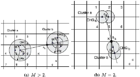
The sensor layer is the bottom and basic layer. For generality, we do not make any assumptions on sensor distribution or node capability, such as location-awareness. Each sensor is assumed to be able to communicate only with its neighbours, i.e., the nodes within its transmission range. During initialization, sensors are self-organized into clusters. Each sensor decides to be either a cluster head or a cluster member in a distributed manner. Sensors with higher residual energy would become cluster heads and each cluster has at most Mb cluster heads, where M is a system parameter. For convenience, the multiple cluster heads within a cluster are called a cluster head group (CHG), with each cluster head being the peer of others. The algorithm constructs clusters such that each sensor in a cluster is one hop away

from at least one cluster head. The FT designed to static

WSNs, and there is no predefined topology to transfer the data from the sensor nodes to sink. Here, all the sensor nodes directly communicate with the sink or simply forwards the data packets to the one-hop neighbour nodes and finally reach to the sink. The existing methods have limitation such as delay, node failure, data redundancy and large amount of energy utilization, since it is using flooding, gossiping, direct communication, etc., to communicate between the nodes. It is the main drawback of this topology and not recommended to mobile WSNs. Upon the arrival of SenCar, each CHG uploads buffered data via MU-MIMO communications and synchronizes its local clocks with the global clock on SenCar via acknowledgement messages. Finally, periodical re-clustering is performed to rotate cluster heads among sensors with higher residual energy to avoid draining energy from cluster heads. Fig 2 describes the SenCar layer with LBC-DDU.

The cluster head layer consists of all the cluster heads. As a fore mentioned, inter-cluster forwarding is only used to send the CHG information of each cluster to SenCar, which contains an identification list of multiple cluster heads in a CHG. Such information must be sent before SenCar departs for its data collection tour. Upon receiving this information, SenCar utilizes it to determine where to stop within each cluster to collect data from its CHG. To collect data as fast as possible, SenCar should stop at positions inside a cluster that can achieve maximum capacity[7][8]. In theory, since SenCar is mobile, it has the freedom to choose any preferred position.

However, this is infeasible in practice, because it is very hard to estimate channel conditions for all possible positions. Thus, we only consider a finite set of locations. To mitigate the impact from dynamic channel conditions, SenCar measures channel state information before each data collection tour to select candidate locations for data collection. We call these possible locations SenCar can stop to perform synchronized data collections polling points. In fact, SenCar does not have to visit all the polling points. Instead, it calculates some polling points which are accessible and we call them selected polling points. In addition, we need to determine the sequence for SenCar to visit these selected polling points such that data collection latency is minimized. Since SenCar has pre-knowledge about the locations of polling points, it can find a good trajectory by seeking the shortest route that visits each selected polling point exactly once and then returns to the data sink.

2.1 MU-MIMO

MU-MIMO can greatly speed up data collection time and reduce the overall latency. Another application scenario emerges in disaster rescue. For example, to combat forest fire, sensor nodes are usually deployed densely to monitor the situation. These applications usually involve hundreds of readings in a short period (a large amount of data) and are risky for human being to manually collect sensed data. A mobile collector equipped with multiple antennas overcomes these difficulties by reducing data collection latency and reaching hazard regions not accessible by human being[1][2][10]. Although employing mobility may elongate the moving time, data collection time would become dominant or at least comparable to moving time for many high-rate or densely deployed sensing applications. In addition, using the mobile data collector can successfully obtain data even from disconnected regions and guarantee that all of the generated data are collected.

3. LOAD BALANCED CLUSTERING

(3)

Page 430

makes the decision on its status based on local information. After running the LBC algorithm, each cluster will have at most M (>1) cluster heads, which means that the size of CHG of each cluster is no more than M. Each sensor is covered by at least one cluster head inside a cluster. The LBC algorithm is comprised of four phases: (1) Initialization; (2) Status claim; (3) Cluster forming and (4) Cluster head synchronization.

3.1 Initialization phase

In the initialization phase, each sensor acquaints itself with all the neighbours in its proximity. If a sensor is an isolated node (i.e., no neighbour exists), it claims itself to be a cluster head and the cluster only contains itself. Otherwise, a sensor, say, si, first sets its status as “tentative” and its initial priority by the percentage of residual energy. Neighbours with the highest initial priorities, which are temporarily treated as its candidate peers. We denote the set of all the candidate peers of a sensor by A.

Fig 3 LBC Algorithm M=2

It implies that once si successfully claims to be a cluster head, its up-to-date candidate peers would also automatically become the cluster heads, and all of them form the CHG of their cluster. si sets its priority by summing up its initial priority with those of its candidate

peers. In this way, a sensor can choose its favourable peers along

with its status decision. Fig. 3b depicts the initialization phase of the example, where M is set to 2, which means that each sensor would pick one neighbour with the highest initial priority as its candidate peer.

3.2 Status claim

In the second phase, each sensor determines its status by iteratively updating its local information, refraining from promptly claiming to be a cluster head. Whether a sensor can finally become a cluster head primarily depends on its priority. Specifically, we partition the priority into three zones by two thresholds, th and tm (th > tm) , which enable a sensor to declare itself to be a cluster head or member, respectively, before reaching its maximum number of iterations. During the iterations, in some cases, if the priority of a sensor is greater than th or less than tm compared with its neighbours, it can immediately decide its final status and quit from the iteration. We call this process self-driven status transition. Also, si will announce

its current candidate peers to be cluster heads by broadcasting a packet including an ID list, which is referred to as the peer-driven status transition.

3.3 Cluster forming

The third phase is cluster forming that decides which cluster head a sensor should be associated with. The criteria can be described as follows: for a sensor with tentative status or being a cluster member, it would randomly affiliate itself with a cluster head among its candidate peersfor load balance purpose. In the rare case that there is no cluster head among the candidate peers of a sensor with tentative status, the sensor would claim itself and its current candidate peers as the cluster heads. Cluster members that receive this message switch to the initialization phase to perform a new round of clustering.

3.4 Synchronization among cluster heads

To perform data collection by TDMA techniques, intra cluster time synchronization among established cluster heads should be considered. The fourth phase is to synchronize local clocks among cluster heads in a CHG by beacon messages. First, each cluster head will send out a beacon message with its initial priority and local clock information to other nodes in the CHG. Then it examines the received beacon Messages to see if the priority of a beacon message is higher. If yes, it adjusts its local clock according to the timestamp of the beacon message. In our framework, such synchronization among cluster heads is only performed while SenCar is collecting data. Because data collection is not very frequent in most mobile data gathering applications, message overhead is certainly manageable within a cluster[2][14].

4 Cluster Head Layer-Connectivity Among CHGs

(4)

Page 431

CHGs. Hence, the inter-cluster communication in LBC-DDUs essentially the communication among CHGs. By employing the mobile collector, cluster heads in a CHG need not to forward data packets from other clusters. Instead, the inter-cluster transmissions are only used to forward the information of each CHG to SenCar.

The inter-cluster organization is determined by the relationship between the inter-cluster transmission range Rt and the sensor transmission range Rs. Clearly, Rt is much larger than Rs. It implies that in a traditional single-head cluster, each cluster single-head must greatly enhance its output power to reach other cluster heads.

However, in LBC-DDU the multiple cluster heads of a CHG can mitigate this rigid demand since they can cooperate for inter-cluster transmission and relax the requirement on the individual output power. Figure 4 Neighbouring distance between clusters. In the following, we first find the condition on Rth at ensures inter-cluster connectivity, and then discuss how the cooperation in a CHG achieves energy saving in output power.

Fig 4 Distance between neighbouring clusters

Consider cluster a. No matter where it is located and how it is oriented, it can completely or partially cover at most six cells. The worst case is that all the sensors in these six cells are in the range of cluster a. Thus, the closest sensor Sk outside of cluster a should be at the right bottommost corner of cell k, which is under cell 5. Cluster heads in a CHG as multiple antennas both in the transmitting and receiving sides such that an equivalent MIMO system can be constructed[6][7][8]. The self-driven cluster head in a CHG can either coordinate the local information sharing at the transmitting side or act as the destination for the cooperative reception at the receiving side. Each collaborative cluster head as the transmitter encodes the transmission sequence according to a specified space-time block code (STBC) to achieve spatial diversity. Compared to the single-input single-output system, that a MIMO system with spatial diversity leads to higher reliability given the same power budget. An alternative view is that for the same receive sensitivity; MIMO systems require

less transmission energy than SISO systems for the same transmission distance. Therefore, given two connected clusters, compared with the single-head structure, in which the inter-cluster transmission is equivalent to a SISO system, the multi-head structure in LBC-DDU can save energy for inter-cluster communication.

4.1 MU-MIMO Uploading

We jointly consider the selections of the schedule pattern and selected polling points for the corresponding scheduling pairs, aiming at achieving the maximum sum of MIMO uplink capacity in a cluster. We assume that SenCar utilizes the minimum mean square error receiver with successive interference cancellation (MMSE-SIC) as the receiving structure for each MIMO data uploading. Based on this receiver, the capacity of a 2 _ 2 MIMO uplink between a scheduling pair ða; bÞ and SenCar located at a selected polling point can be expressed as follows.

where ha and hb are two 2 _ 1 channel vectors between cluster heads a and b and SenCar at ~, respectively, Pt is the output power of a sensor for transmission range Rs, and N0 is the variance of the back-ground Gaussian noise. The MMSE-SIC receiver first decodes the information from a, treating the signals of b as the interference. Then, it cancels the signal part of a from the received signals. The remaining signal part of b only has to contend with the background Gaussian noise. Once the selected polling points for each cluster are chosen, SenCar can finally determine its trajectory. The moving time on the trajectory can be reduced by a proper visiting sequence of selected polling points. Since SenCar departs from the data sink and also needs to return the collected data to it, the trajectory of SenCar is a route that visits each selected polling point once. This is the well-known travelling salesman problem (TSP). Since SenCar has the knowledge about the locations of polling points, it can utilize an approximate or heuristic algorithm for the TSP problem to find the shortest moving trajectory among selected polling points, e.g., the nearest neighbour algorithm[10][11]

5. Performance Evaluations

[image:4.612.47.289.341.474.2]

(5)

Page 432

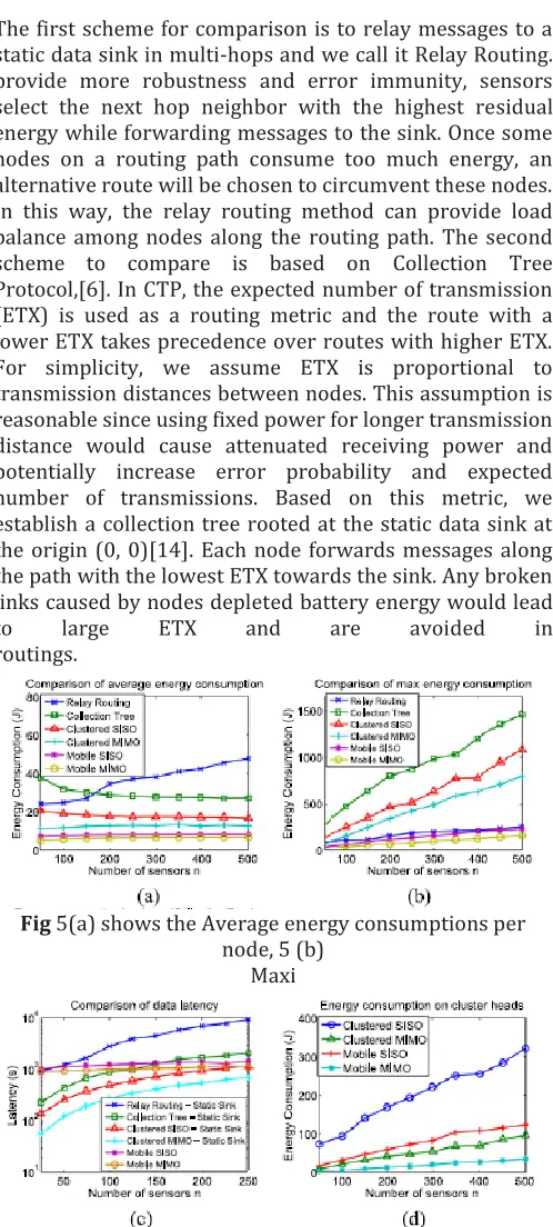
The first scheme for comparison is to relay messages to a static data sink in multi-hops and we call it Relay Routing. provide more robustness and error immunity, sensors select the next hop neighbor with the highest residual energy while forwarding messages to the sink. Once some nodes on a routing path consume too much energy, an alternative route will be chosen to circumvent these nodes. In this way, the relay routing method can provide load balance among nodes along the routing path. The second scheme to compare is based on Collection Tree Protocol,[6]. In CTP, the expected number of transmission (ETX) is used as a routing metric and the route with a lower ETX takes precedence over routes with higher ETX. For simplicity, we assume ETX is proportional to transmission distances between nodes. This assumption is reasonable since using fixed power for longer transmission distance would cause attenuated receiving power and potentially increase error probability and expected number of transmissions. Based on this metric, we establish a collection tree rooted at the static data sink at the origin (0, 0)[14]. Each node forwards messages along the path with the lowest ETX towards the sink. Any broken links caused by nodes depleted battery energy would lead

to large ETX and are avoided in

routings.

Fig 5(a) shows the Average energy consumptions per

node, 5 (b) Maxi

To justify our choice of mobile data collections, we also compare the geographical energy distribution between Collection Tree and mobile MIMO. For demonstration purposes, we set n ¼ 200 and draw the heat map of energy consumption. We observe that more energy is consumed

with the Collection Tree method especially on nodes near the data sink represented by the bright spots .These nodes may become congested bottlenecks and jeopardize the operation of the network. Although mechanisms in Collection Tree can find a better route by adapting to ETX metrics, congestion is inevitable due to the physical locations of these nodes. In contrast, the mobile MIMO method results in much less energy consumption and even distribution across the sensing field .

REFERENCES

[1] B. Krishnamachari, Networking Wireless Sensors. Cambridge, U.K.: Cambridge Univ. Press, Dec. 2005.

[2] R. Shorey, A. Ananda, M. C. Chan, and W. T. Ooi, Mobile, Wireless, Sensor Networks. Piscataway, NJ, USA: IEEE Press, Mar. 2006.

[3] W. C. Cheng, C. Chou, L. Golubchik, S. Khuller, and Y. C. Wan, “A coordinated data collection approach: Design, evaluation, and comparison,” IEEE J. Sel. Areas Commun., vol. 22, no. 10, pp. 2004– 2018, Dec. 2004.

[4] K. Xu, H. Hassanein, G. Takahara, and Q. Wang, “Relay node deployment strategies in heterogeneous wireless sensor networks,” IEEE Trans. Mobile Comput., vol. 9, no. 2, pp. 145–159, Feb. 2010.

[5] E. Lee, S. Park, F. Yu, and S.-H. Kim, “Data gathering mechanism with local sink in geographic routing for wireless sensor networks,” IEEE Trans. Consum. Electron., vol. 56, no. 3, pp. 1433– 1441, Aug. 2010.

[6] Y. Wu, Z. Mao, S. Fahmy, and N. Shroff, “Constructing maximum- lifetime data-gathering forests in sensor networks,” IEEE/ ACM Trans. Netw., vol. 18, no. 5, pp.

1571–1584, Oct. 2010.

[7] X. Tang and J. Xu, “Adaptive data collection strategies for lifetime- constrained wireless sensor networks,” IEEE Trans. Parallel Distrib. Syst., vol. 19, no. 6, pp. 721–7314, Jun. 2008.

[image:5.612.39.288.96.648.2]

(6)

Page 433

[9] O. Younis and S. Fahmy, “Distributed clustering in ad-hoc sensor networks: A hybrid, energy-efficient approach,” in IEEE Conf. Comput. Commun., pp. 366–379, 2004.

[10] D. Gong, Y. Yang, and Z. Pan, “Energy-efficient clustering in lossy wireless sensor networks,” J. Parallel Distrib. Comput., vol. 73, no. 9, pp. 1323–1336, Sep. 2013.

[11] A. Amis, R. Prakash, D. Huynh, and T. Vuong, “Max-min d-clusterformation in wireless ad hoc networks,” in Proc. IEEE Conf. Comput. Commun., Mar. 2000, pp. 32–41.

[12] A. Manjeshwar and D. P. Agrawal, “Teen: A routing protocol for enhanced efficiency in wireless sensor

networks,” in Proc. 15th Int. IEEE Parallel Distrib. Process. Symp., Apr. 2001, pp. 2009–2015.

[13] Z. Zhang, M. Ma, and Y. Yang, “Energy efficient multi-hop polling in clusters of two-layered heterogeneous sensor networks,” IEEE Trans. Comput., vol. 57. no. 2, pp. 231–245, Feb. 2008.