Evaluation of spatial audio reproduction
methods (part 2) : analysis of listener
preference
Francombe, J, Brookes, T, Mason, R and Woodcock, J
10.17743/jaes.2016.0071
Title
Evaluation of spatial audio reproduction methods (part 2) : analysis of
listener preference
Authors
Francombe, J, Brookes, T, Mason, R and Woodcock, J
Type
Article
URL
This version is available at: http://usir.salford.ac.uk/id/eprint/41952/
Published Date
2017
USIR is a digital collection of the research output of the University of Salford. Where copyright
permits, full text material held in the repository is made freely available online and can be read,
downloaded and copied for noncommercial private study or research purposes. Please check the
manuscript for any further copyright restrictions.
JournaloftheAudioEngineeringSociety Vol.65,No.3,March2017
DOI:https://doi.org/10.17743/jaes.2016.0071
Evaluation of Spatial Audio Reproduction Methods
(Part 2): Analysis of Listener Preference
JON FRANCOMBE1
, TIM BROOKES,1AES Member, RUSSELL MASON,1AES Member, AND
JAMESWOODCOCK2
1InstituteofSoundRecording,UniversityofSurrey,Guildford,UK
2AcousticsResearchCentre,UniversityofSalford,Salford, UK
Itisdesirabletodeterminewhichofthemanydifferentspatialaudioreproductionsystems listenersprefer,andtheperceptualattributesthataremostimportanttolistenerexperience, sothatfuturesystemscanbeperceptuallyoptimized.Apairedcomparisonpreferencerating experimentwasperformedalongsideafreeelicitationtaskforeightreproductionmethods (consumerandprofessionalsystemswithawiderangeofexpectedquality)andsevenprogram items (representative of potential broadcastmaterial). The experiment was performed by groupsofexperienced andinexperienced listeners. ThurstoneCaseV modelingwasused toproducepreferencescales. Bothlistenergroupspreferredsystemswithincreasedspatial content;nine-andfive-channelsystemsweremostpreferred.Theuseofelicitedattributeswas analyzedalongsidethepreferenceratings,resultinginanapproximatehierarchyofattribute importance:threeattributes(amountofdistortion,outputquality, andbandwidth)werefound tobeimportant fordifferentiatingsystemswheretherewasa largepreferencedifference; sixteenwerealwaysimportant (mostnotablyenveloping andhorizontal width);and seven wereusedalongsidesmallpreferencedifferences.
0 INTRODUCTION
There is a wide range of spatial audio reproduction methods used for domestic or professional audio replay. Systems include mono and two-channel stereo, channel-based surround sound methods (5.1, 7.1, 9.1, 11.1, and 22.2 [1] are all used domestically or within the audio in-dustry), “one box” solutions such as sound bars, and re-production over headphones. With such a wide range of methods in use, it is important to discover what aspects of spatial audio reproduction particularly enhance the listener experience.
A previous study by the authors [2] identified the percep-tual attributes that contribute to preference judgments made between alternative reproduction systems. The research de-scribed in the current paper aimed to determine which of these attributes are most important to listeners—that is, which of them have a strong relationship with listener pref-erence. With this knowledge, these attributes can then be targeted in the design of new reproduction systems and the improvement of existing ones, and perceptual models of the important attributes can be developed and used to meter and optimize spatial audio reproduction. The problem was approached from two directions: determining listener pref-erence for certain systems and ascertaining the perceptual characteristics of the differences between the systems. By
collecting both quantitative and qualitative data, the rela-tionship between the attributes and preference scores could be investigated. This facilitated analysis of the perceptual attributes that most contribute to creating a positive listener experience.
1 EXPERIMENT BACKGROUND
There have been previous attempts to understand the re-lationship between audio attributes and listener preference. Choisel and Wickelmaier [3] performed a spatial audio elicitation experiment and determined a set of eight at-tributes:width,elevation,spaciousness,envelopment,
dis-tance,brightness,clarity, andnaturalness. They then
coefficients and the percepts to which they relate. As each feature in the model relates to a complex combination of multiple perceptual attributes that have been combined in the dimension-reduction stage, it is not possible to assess the coefficients and thereby determine the contribution of a single attribute to preference.
Zacharov and Koivuniemi [5] also elicited a set of at-tributes producing twelve scales:sense of direction,sense
of depth,sense of space,sense of movement,penetration,
distance to events,broadness,naturalness,richness,
hard-ness,emphasis, andtone color. They performed a
prefer-ence mapping experiment, collecting attribute ratings for eight reproduction systems (including mono, stereo, five-channel, eight-five-channel, and crosstalk-cancelled binaural systems) on scales with a resolution of 100 points using a single stimulus presentation. They analyzed the correla-tion between the scales and found that some attributes were significantly correlated. A partial least squares regression (PLS-R) was performed to map the attribute ratings to pref-erence scores; a model with four components explaining 71% of the variance in the scores was found to be most suitable, with the following attributes contributing most significantly to the prediction:sense of movement,sense of
depth,direction×distance,broadness×distance,
broad-ness×tone color, anddepth×naturalness. In this case,
the PLS-R analysis combined more than one attribute to give an interaction term that is both relatively difficult to interpret and likely to be less generalizable (e.g., what does the combination ofdepth×naturalness mean and under what circumstances is it important?).
In the above studies, the use of statistical dimension-reduction techniques has been problematic. While the re-sults may have provided some information on the relation-ship between attributes and preference, they are not suf-ficient to provide clear guidance for future researchers on what attribute should be investigated or optimized.
In the current study an alternative approach was taken that avoided the need to collect ratings on a large num-ber of scales and also avoided the use of data reduction techniques such as PCA. An attribute elicitation exper-iment was performed alongside a preference rating task in an attempt to produce only those attributes that made a significant contribution to listener preference. Partici-pants were asked to give preference ratings and, on the same screen, to type their reasons for making a partic-ular judgment. The attribute elicitation aspects of this work are reported by Francombe et al.[2]. The attribute sets produced (by experienced and inexperienced listen-ers) were large (a total of 51 attributes—27 and 24 by the experienced and inexperienced listeners respectively, with some overlap between the sets). The preference ratings (which are analyzed in this paper) and elicited data were used in conjunction to determine particularly important attributes.
1.1 Research Questions
The research questions addressed in this study were as follows.
1. What spatial audio reproduction methods do listen-ers prefer?
2. Which attributes are most important to listener expe-rience and should therefore be used in further eval-uations?
It was also considered desirable to investigate the effect of listener experience on the answers to these questions. De-scriptive analysis experiments often rely solely on experi-enced listeners for scale development and on inexperiexperi-enced listeners for preference ratings [6, p. 346]; for example, Rumsey et al.[7] determined the relationship between the preference of inexperienced listeners and quality judgments made by experienced listeners. However, in this case it was considered beneficial to discover how inexperienced listen-ers perceive spatial audio stimuli, as such listenlisten-ers account for the majority of domestic spatial audio consumption.
The methodology for the paired comparison preference rating experiment is described in Sec. 2. The preference results are detailed in Sec. 3, and the relationship between the elicited attributes and listener preference is discussed in Sec. 4. Finally, the outcomes from this work are discussed and concluded in Sec. 5.
2 PREFERENCE RATING EXPERIMENT METHODOLOGY
The methodology employed for the preference rating experiment is described in the following sections.
2.1 Stimuli and Participants
One limitation of previous studies is the restricted range of reproduction systems tested. It is not possible to test every conceivable reproduction method, especially as new systems are developed; however, it is desirable to future-proof experiment results to as great a degree as possible by including a wide range of systems. It is also necessary to select program material items that are representative of broadcast content and also able to reveal the differences between reproduction systems.
In this study eight reproduction methods were used: headphones, low-quality mono (a small computer loud-speaker), mono, stereo, 5-channel, 9-channel, 22-channel, and ambisonic cuboid. These methods were selected to cover a range of loudspeaker counts, positions, and ex-pected quality. More details about the reproduction methods are given by Francombe et al.[2].
reproduction system using a production technique that is typical for that system (including spatial microphone tech-niques, amplitude panning, ambisonic decoding, and binau-ral recording [8]). It is therefore not possible to completely separate the reproduction method from the production tech-nique used; however, as a range of techtech-niques were used for each reproduction system, the results averaged across stimuli retain some independence between the production technique and the reproduction method. Hence, the results can still be used to show the magnitudes of preference for different systems (as discussed in Sec. 3.4), and verbal elic-itation alongside preference judgments allows analysis of why particular systems were preferred.
The experiment was performed by two groups of partic-ipants: seven experienced listeners and eight inexperienced listeners. The experienced listeners were fourth year un-dergraduate students on the Music and Sound Recording course at the University of Surrey, Guildford, UK, who had all completed a module in technical ear training and had critical listening experience in recording studios. The in-experienced listeners were current students or recent grad-uates in a range of disciplines. None of the inexperienced listeners had specific technical ear training, although they may have had a musical background and/or have partici-pated in listening tests before.
2.2 Methodology
The listening test was run using a software user interface with multiple pages created in Max/MSP. Each experiment session was preceded by a familiarization stage, again using a bespoke Max/MSP interface. When participants switched between stimuli (in either interface) the position in the au-dio excerpt was maintained to enable easier comparisons. It should be noted that comparisons featuring the head-phone reproduction meant that participants had to put on and remove the headphones when switching between re-production methods, introducing a longer delay than for comparisons not involving the headphones.
All judgments for a single program item were made in one test session; therefore, a total of seven test sessions (each including a familiarization stage and the main test) were performed by each participant. The program items were presented in a different random order for each partic-ipant.
2.2.1 Familiarization Task
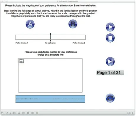
[image:4.585.300.530.44.240.2]Before each test session participants were asked to listen to all of the reproduction methods for the program item under test so that they could learn and understand the full range of stimuli that they would hear in the session and therefore use the rating scale appropriately. If participants were not aware of the full range of reproduction methods before undergoing the test, it is possible that they might give a high preference rating for one stimulus over another, before auditioning a stimulus pair with an even greater difference, leaving no room on the scale to indicate this. The wording for the familiarization task given in the instructions was as follows.
Fig. 1. Interface for the preference rating and free elicitation task.
“In the test stage, you will be asked to indicate the mag-nitude of your preference when comparing a pair of audio stimuli. There will be a total of 31 pairs in each session. Be-fore the test, you will be asked to listen to all of the stimuli that you will hear during the test. Use this familiarization to get an idea of the range of stimuli, and of how much you prefer some to others, so that you can express the magni-tude of your preference appropriately during the test. For example, in the test, within one pair you might have only a slight preference for one of the stimuli over the other; within another pair you might have a very large preference for one stimulus over the other. After listening to the stimuli on the familiarization page, you should be aware of the full range of magnitudes of preference that you are likely to experience during the test, and should therefore be able to rate these accordingly.”
The user interface displayed eight buttons, and the repro-duction methods were randomly assigned to these. Where participants were required to wear headphones, this was in-dicated by a headphone icon next to the appropriate button.
2.2.2 Main Test
The stimuli were presented to participants in a paired comparison paradigm with continuous ratings. The paired comparison methodology was selected as it allowed direct comparison between two stimuli, facilitating the differential elicitation aspect of the study. Paired comparisons were also considered to be easier for participants to make compared to, say, a multiple stimulus test. A continuous scale rating was used since, although this is more demanding to perform than a forced choice, it allows more fine-grained analysis of the difference between stimuli [9] and can be converted to binary judgments if necessary.
vertical line. With eight reproduction methods there is a to-tal of (82)=28 comparisons. Three of these comparisons— selected at random for each of the program items but kept the same for all participants—were repeated to facilitate analysis of participant reliability; this resulted in a total of 31 judgments per program item for each participant. In each session, the stimulus combinations were presented in a ran-dom order and the two stimuli were assigned ranran-domly to buttons A and B. A free elicitation was performed along-side the preference rating task: participants were asked to describe the reasons for giving a particular preference rating [2].
The wording of the preference rating task in the instruc-tions given to participants was as follows.
“Each test session consists of 31 pages. On each page there is a pair of stimuli (labelled A and B). Please listen to the two stimuli and indicate which you prefer, and the magnitude of your preference, on the scale. Bear in mind the full range of stimuli that you heard in the familiarization and try to position the slider appropriately, where: far left indicates that you prefer stimulus A to stimulus B and that the magnitude of your preference is as great as you are likely to experience throughout the test session; far right indicates that you prefer stimulus B to stimulus A and that the magnitude of your preference is as great as you are likely to experience throughout the test session; immediately to the left or right of center indicates the smallest magnitude of preference, for stimulus A (left) or B (right); and center indicates no preference for either A (left) or B (right). Please note that you must move the slider at least once before you can continue to the next page. If you’d like to leave the slider in the middle of the scale, just move it away and then back.”
The interface also showed the waveform of the audio; participants were able to select a short section of the excerpt to loop so that they could repeatedly listen to sections that highlighted differences that they felt to be important.
3 RESULTS
The data preprocessing, analysis of participant reliabil-ity, and analysis of preference results are presented in the following sections.
3.1 Data Preprocessing
To gain an overview of the range of the preference scale that participants were using, box plots of participant re-sponses (pooled over all reproduction methods and pro-gram items) were plotted (Fig. 2). The box plots show the median, lower and upper quartiles, and range of the data, as well as any outliers. The notches can be used to determine significant differences in the median value; where notches do not overlap, the medians can be considered to be signif-icantly different [10]. The extremes of the preference scale are indicated by−50 and 50, which indicate a preference for stimulus A and stimulus B respectively. In the experi-ment, the assignment of each stimulus in a pair to buttons A or B on the interface was randomized. Therefore, when
I1 I2 I3 I4 I5 I6 I7 I8 E1 E2 E3 E4 E5 E6 E7
−50 0 50
Participant
[image:5.585.305.539.44.164.2]Preference score
Fig. 2. Box plots of all responses by each participant. Partici-pant prefix “E” indicates an experienced listener; “I” indicates an inexperienced listener.
generating this plot some data were inverted so that the A–B ordering for each pair was consistent across all tests. Thus, the slight positive offset in the scores seen in Fig. 2 does not indicate a bias towards stimulus B but, rather, a preference for the higher channel count systems, that tend (arbitrarily) to come second in the modified comparison order more often (79% of comparisons). It can be seen that the expe-rienced listeners tended to use the full range of the scale, while the inexperienced listeners exhibit a high degree of inter-listener variance, with some participants (notably I2, I4, I5, and I6) using a reduced scale range. Consequently, the preference values were scaled for each participant by dividing each score by the standard deviation of the scores for that participant (az-score transformation was not used as this includes mean-centering; in this case, centering the data was not appropriate as the center point of zero has a particular meaning, i.e., no preference). However, even with the application of the scaling, the very small range of results given by I2 is likely to mean that the results are noisy and unreliable (and in fact these results were discarded due to their unreliability—see Sec. 3.2.2).
3.2 Participant Reliability
3.2.1 Circular Error Percentage
One measure of the participants’ ability to perform a paired comparison task is the circular error percentage. The responses for each possible triad of stimuli should exhibit transitivity; that is, if A → Band B→ C, then A → C
should hold (where→ is read as “is preferred to”) [11]. The circular error percentage is the percentage of all pos-sible triads of paired comparisons (given by (S3) whereSis the number of stimuli) for which the ratings are intransitive. The mean circular error percentages across all program ma-terial items were 5.55% and 3.46% for the inexperienced and experienced listeners respectively. No individual par-ticipant or program material item exceeded a mean circular error percentage of 10%.
3.2.2 Repeat Judgments
I1 I2 I3 I4 I5 I6 I7 I8 E1 E2 E3 E4 E5 E6 E7 0
0.2 0.4 0.6 0.8 1 1.2 1.4
Participant
Mean a
b
sol
u
te difference (scaled)
[image:6.585.299.534.43.176.2]33% 38% 10% 19% 19% 38% 19% 24% 24% 29% 10% 24% 19% 33% 10%
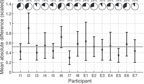
Fig. 3. Mean absolute difference between repeated judgments (scores scaled as described in Sec. 3.1). Error bars show 95% confidence intervals calculated using thet-distribution. The gray horizontal line shows the grand mean across all participants. The dark area of each pie chart shows the percentage of preference judgments that were changed between replicates. Participant pre-fix “E” indicates an experienced listener; “I” indicates an inexpe-rienced listener.
the mean absolute difference between the first and second judgments, averaged across all 21 items for each participant. The horizontal line shows the mean across participants. One participant (I2) has a difference significantly greater than the mean; this is unsurprising given the limited range of re-sponses mentioned above. Fig. 3 also shows the percentage of judgments in which a different preference was speci-fied (i.e., one reproduction method was preferred in the first judgment and the other method preferred in the second judgment, or a “no preference” judgment was changed to a preference in either direction). Three inexperienced par-ticipants (including I2) have values above 25%. The mean percentage is slightly lower for the experienced listeners (21% and 25% for experienced and inexperienced listen-ers respectively); two experienced listenlisten-ers gave revlisten-erse judgments in over 25% of cases.
As the replicates were selected at random, it is possi-ble that those selected were particularly difficult (or easy) comparisons for which to make a preference judgment; for example, the program items selected may just have been very similar, making the judgment difficult. Unless every test item is repeated, this cannot be completely avoided; however, it was felt that this was a necessary trade-off to ensure that the experiment could be performed in a suitable time frame while allowing for analysis of listener reliability. To determine whether any of the selected replicates were found to be particularly difficult to perform, the mean ab-solute difference for each of the 21 replicates was plotted (Fig. 4), again alongside the percentage of judgments that were changed between the first and second replicate. The plot shows that there are no significant differences between the performance on each of the replicate stimuli. However, it is interesting to interpret these results alongside the per-centage of changed judgments. When the mean absolute difference is low but the percentage of judgments changed is high (e.g., replicate 3: brass quintet, headphones versus 5-channel), this suggests that it was difficult to determine a
1 2 3 4 5 6 7 8 9 10 11 12 13 14 15 16 17 18 19 20 21
0 0.2 0.4 0.6 0.8 1 1.2 1.4
Replicate number
Mean a
b
sol
u
te difference (scaled)
0% 53% 40% 7% 7% 27% 33% 20% 0% 33% 40% 60% 33% 0% 20% 0% 20% 20% 20% 7% 47%
Fig. 4. Mean absolute difference between repeated judgments for each repeated stimulus (scores scaled as described in Sec. 3.1). Error bars show 95% confidence intervals calculated using thet -distribution. The gray horizontal line shows the grand mean across all replicates. The dark area of each pie chart shows the percentage of preference judgments that were changed between replicates.
preference for either stimulus. Therefore, small preference ratings were given in either direction and a small differ-ence in rating could lead to a change in preferdiffer-ence. In other cases, a relatively large mean absolute difference was accompanied by a high percentage of changed judgments (e.g., replicate 12: jazz quintet, stereo versus 5-channel), indicating that participants found it difficult to make judg-ments for this stimulus. Finally, a relatively large mean absolute difference accompanied by a small percentage of changed judgments (e.g., replicate 20: film excerpt, low-quality mono versus ambisonic cuboid) indicates that par-ticipants were confident of the method that was preferred but unsure of the magnitude of their preference judgments. The results on the whole indicate that the replicates cover a wide range of difficulty of judgment and therefore serve as a useful indicator of subject reliability.
Based on the evidence presented above (i.e., a relatively large mean absolute difference, high percentage of changed judgments, and small range of scale use), it was determined that the results from listener I2 were unreliable; they were therefore discarded for all further analysis of preference.
The repeat judgments were included in the experiment design solely to enable analysis of listener reliability; they were therefore removed from the data before any further analysis to maintain a balanced dataset. In every case, the first judgment was used.
3.3 Preference for Reproduction Methods
Thurstone Case V modeling [12] was used to convert the paired comparison data into a preference scale for the different reproduction methods, using the code presented by Tsukida and Gupta [13]. The model assumes that the relative magnitudes of preferences for the stimuli can be determined from the percentage of times that one stimulus is selected over another in a paired comparison task.
[image:6.585.48.281.45.181.2]0 0.1 0.2 0.3 0.4 0.5 0.6 0.7 0.8 0.9 1
Reproduction method
Mean normalized scale val
u
e
LowQual Mono Cuboid
Headphones Stereo 22−chan 5−chan 9−chan
[image:7.585.304.540.41.294.2]Inexperienced listeners Experienced listeners
Fig. 5. Preference scale created using Thurstone Case V model with raw scores for experienced and inexperienced listeners. Con-fidence intervals show bootstrapped 95% conCon-fidence intervals cal-culated over 50 iterations.
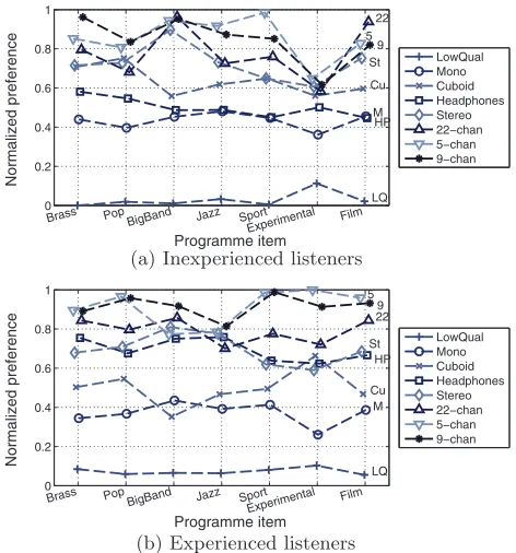
as the mean of the scale points across all of the samples, and confidence intervals calculated using the normal dis-tribution. In this case, approximately 50% of the data were used in each iteration (25 out of 49 judgments for each re-production method), and the procedure was repeated for 50 random samples. For comparisons in which one stimulus was always preferred over the other, an offset the equivalent size of a no preference judgment was added to the stimu-lus that was never preferred, and taken off the stimustimu-lus that was always preferred, in order to allow computation of the scale (the inverse normal distribution function is used to determine scale values, returning an infinite value for a probability of 1 or 0; the correction avoided this problem). The Thurstone scale values were normalized to the range 0–1 (over all iterations and both subject types) before taking the mean across bootstrap iterations. The resulting scales for the experienced and inexperienced listeners are shown in Fig. 5, ordered according to the experienced listeners’ preference.
The confidence intervals are small, suggesting that the scale values are reliable and that the reproduction meth-ods can clearly be differentiated; the only exception to this are small differences in the inexperienced listeners’ results between the 5-channel and 9-channel methods and the 22-channel and stereo methods. The results show that the low-quality mono reproduction method is clearly the least preferred by both sets of listeners, followed by the monophonic reproduction. This suggests that both types of listener prefer the presence of increased spatial information. However, it is interesting to note that preference does not in-crease monotonically with channel count. The experienced listeners display only a marginal preference for the cuboid reproduction over mono, while the inexperienced listen-ers display only a small preference for headphones. For both groups of listeners, the 22-channel reproduction was preferred less than the 5- and 9-channel methods. The inex-perienced listeners distinguished less between the different surround sound methods, although the pattern of preference is similar to that of the experienced listeners.
0 0.2 0.4 0.6 0.8 1
LQ M Cu
HP St
22 5
9
Programme item
N
ormalized preference
Brass Pop
BigBand Jazz SportExperimental Film
LowQual Mono Cuboid Headphones Stereo 22−chan 5−chan 9−chan
(a) Inexperienced listeners
0 0.2 0.4 0.6 0.8 1
LQ M Cu
HP St
22 5
9
Programme item
N
ormalized preference
Brass PopBigBand Jazz Sport Experimental
Film
LowQual Mono Cuboid Headphones Stereo 22−chan 5−chan 9−chan
(b) Experienced listeners
Fig. 6. Preference scale, broken down by stimuli, created using Thurstone Case V model with raw scores, for experienced and inexperienced listeners.
3.3.1 Preference by Program Item
In order to determine the effect of program item on lis-tener preference for the reproduction methods, the Thur-stone scaling was repeated with the data broken down by program item. Due to the reduced number of cases, the boot-strapping procedure was not performed; however, the small confidence intervals seen in the results presented above suggest that the preference scaling is consistent.
Fig. 6 shows the preference scale values for each repro-duction method (denoted by line shade and marker shape) for each program material item. Lines that intersect indicate different rank orders of reproduction methods depending on the program item. There is some variance in preference for the different program items; however, the reproduction methods themselves have a greater effect on the results. This is confirmed by analyzing the rank correlation using Kendall’s coefficient of concordance (W), which measures the agreement between multiple sets of ranks [14]. In this case,W=0.91 andW=0.90 for the inexperienced and ex-perienced listeners respectively, indicating high agreement between the rank orders for each program item.
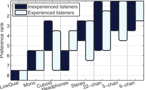
[image:7.585.54.288.44.194.2]8 7 6 5 4 3 2 1
LowQual Mono CubHeadphonesoid Stereo22−chan 5−chan 9−chan
Preference rank
[image:8.585.49.282.45.188.2]Inexperienced listeners Experienced listeners
Fig. 7. Range of preference ranks for each reproduction method (experienced and inexperienced listeners).
to a lack of familiarity with the type of program material resulting in generally lower preference.
For the experienced listeners, the cuboid exhibited a rel-atively low score for the big band reproduction and a high score for the experimental music (which was specifically designed for ambisonic replay). The 5-channel reproduc-tion of the big band program item received a relatively low preference rating. The mono reproduction of the experi-mental music received a low preference score, indicating that spatial content was important to the experienced lis-teners for this program item—this could be influenced by the pronounced movement within the sound sources in this item.
Some reproduction methods exhibited more variable preference ratings than others with different program ma-terial. The range of rank positions that each reproduction method achieved is displayed in Fig. 7. For both groups of listeners, the low-quality mono reproduction was always ranked eighth out of eight. For the inexperienced listen-ers, the 22-channel method shows the highest variance, ranking between fifth and first depending on the program material. For the experienced listeners, the 5-channel, 22-channel, stereo, and cuboid methods all have a high vari-ance (four different rank positions over the seven program items). The 9-channel method consistently received high preference scores—it was always ranked in the top three for both listener groups (and first or second for the experi-enced listeners).
3.4 Discussion
The results presented above show a clear benefit of au-dio systems that provide spatial information, with stereo preferred to mono, and surround sound preferred to stereo. However, the trends in preference for the surround sound systems are less clear. The results show little difference between the 5-channel and 9-channel reproduction meth-ods, suggesting that height content is not always beneficial, or results in little increase in preference—although there are specific program items where the preference score is increased with the addition of height channels. The 22-channel system has the highest loudspeaker count but for
most program items scores lower than the 5- and 9-channel methods.
The experienced and inexperienced listeners tended to be in reasonably strong agreement, although the experi-enced listeners could discriminate between the most pre-ferred systems slightly more. The main differences were in the headphone reproduction (preferred considerably by the experienced listeners) and the ambisonic reproduction (preferred by the inexperienced listeners).
It should be noted that the production of the program items was inextricably linked to the reproduction methods in this experiment (albeit using representative production techniques); an argument could be made that 22-channel was less preferred as the content was less suitable. There is generally less experience in producing 22-channel content, which may mean that the full capabilities of this system have not been achieved. Therefore, it is not possible to conclude that there will never be a benefit of 22-channel reproduction; however, based on these results, any prefer-ence shown over five or nine loudspeakers appears to be relatively small. This finding is supported by the results presented by Silzle et al.[15], who found only small dif-ferences in ratings of quality for 5-channel, 9-channel, and 22-channel reproductions in an experiment with no ref-erence. Where a 22-channel reference was included, the differences between reproduction methods were more pro-nounced, with higher quality ratings for the higher channel count reproductions. Further analysis in this paper will fo-cus on the reasons that listeners gave for making preference judgments, enabling the results to be used to determine the perceptual advantages and disadvantages of the particular methods.
4 DETERMINING THE IMPORTANT ATTRIBUTES
The second research question presented in Sec. 1.1 ad-dressed the need for determining the attributes that are most important to listener experience. It is desirable to know which attributes are important so that they can be used for evaluation in listening tests, in meters for use by content producers, and in algorithms for the optimization of spatial audio systems.
One way to determine which of the attributes are of particular importance would be to collect and statistically analyze ratings of stimuli on every attribute scale. Such analyses might include determination of the correlation be-tween attributes, assessment of listener agreement on each attribute, or observation of the relationship between the at-tributes and preference. However, due to redundancy in the attribute set, it is inefficient to rate every attribute; even when attempting to elicit unique attributes, the produced terms often still overlap. The results of dimension-reduction analysis can also be difficult to interpret (as discussed in Sec. 1). For example, multiple attributes or attribute inter-actions may be represented on a single dimension.
experiment in which participants were requested to choose the most relevant attribute for each of a set of stimuli. Frequency of attribute use was employed to select four attributes from the original set of twelve; the selection was shown to be suitable in the subsequent rating experiment, as a principal component analysis showed that two dimensions accounted for 90% of the variance in the ratings, and two of the four attributes were highly correlated.
In this case, the collection of preference ratings alongside free elicitation responses facilitates analysis of the attribute use, allowing selection of a subset of important attributes. An attribute can be considered important [6, pp. 343–346] if:
• It is used and understood by all participants; and
• It allows differentiation between the stimuli under test.
The analyses described below were performed to deter-mine which of the attributes meet these criteria and should therefore be investigated further. First, a mapping between the free elicitation data and resultant attributes was per-formed so that attribute use could be considered with re-lation to particular stimuli (Sec. 4.1). This was followed by analysis of the attributes against the two criteria. The percentage of participants that used each attribute is ana-lyzed in Sec. 4.2. The discriminatory power of the attributes is assessed in Sec. 4.3 by looking at the frequency of use of the attributes alongside different preference judgments. Definitions of the attributes used in this study are given by Francombe et al.[2]
4.1 Free Elicitation Data to Attribute Mapping
The attributes considered below were determined by a free elicitation, an automatic text clustering process to re-duce redundancy, and then group discussions in which the algorithmically-generated clusters were put into sets, which were subsequently labelled and defined [2].
To facilitate analysis of the attributes, each response from the free elicitation was mapped to the attribute to which it ultimately contributed by: (i) identifying the cluster in which the response was included (by the automatic cluster-ing algorithm); and (ii) identifycluster-ing the attribute to which that cluster ultimately contributed after the cluster-setting and attribute labelling procedure.
However, this process can fail to map some responses for the following reasons.
1. An incorrectly-clustered term may have remained in a cluster that eventually contributed to an attribute, resulting in an incorrect mapping between response and attribute.
2. Some of the automatically produced clusters were discarded. Subsequent listening to audio record-ings of the elicitation group discussions identified two main reasons for discarding clusters: (i) the re-sponses were not useful, i.e., they were meaning-less or ambiguous; or (ii) items in a cluster were
0 10 20 30 40 50 60 70 80 90 100
Percentage of participants (%)
Pos. of so
u nd Clarity S u rro u nding RealismDistance
Rich. of so
u nd O u tp u t q u al. Headphones Bass Harshness Immersion
Can’t hear diff.
Detail
Ease of list.
Discerna b ility Prominence V ol u me Targetting Spat. b al.
Phys. react.Odd so
u nds EchoTre b le Emot. react.
Subject 1
Subject 3
Subject 4
Subject 5
Subject 6
Subject 7
Subject 8
(a) Inexperienced listeners
0 20 40 60 80 100
Percentage of participants (%)
Realism
Amo
u
nt of dist.
Depth of field
EnvelopingSpect. clar.
Ov. spect. b al. Spat. nat u ral. Hor. width
Lev. of rever
b
Spat. clar. BandwidthPhasinessSpect. res.
Sense of space
Spat. open.
S
ub
j. q
u
al. of rever
b
Ov. level
Perc. trans. q
u
al.
Ov. s
ub
j. pref.
Spat. mov.Dyn. rangeSpat.
b
al.
Real. of rever
b
A
u
di
b
. of comp.
Phys. sensation
Ens.
b
alance
Percept. of noise
Subject 1
Subject 2
Subject 3
Subject 4
Subject 5
Subject 6
Subject 7
[image:9.585.306.538.44.146.2](b) Experienced listeners
Fig. 8. Percentage of participants that used terms contributing to each attribute. Each bar is proportioned according to the number of times each participant used a term contributing to the corre-sponding attribute.
relevant to two or more attributes that already had clearly defined groups. For the experienced listen-ers, 58 out of 228 clusters were discarded (25.4%); the remaining 170 clusters accounted for 77.8% of the responses from the free elicitation experiment (1531 from 1967). For the inexperienced listeners, 95 out of 244 clusters were discarded (38.9%); the remaining 149 clusters accounted for 56.4% of the responses from the free elicitation experiment (1281 from 2270). It should be noted that these figures include the results given by inexperienced partici-pant 2 (which were discarded from the preference analysis in this paper), but do not include identical responses given in the free elicitation (which were removed before the automatic clustering).
Despite the discarding of some clusters, analysis of the remaining data can still highlight important attributes. There is a large proportion of the data available, and removal of meaningless responses, i.e., those that participants agreed did not describe the listening experience in a valuable man-ner, is not damaging—in fact, it is potentially beneficial to showing trends. Furthermore, removal of responses that would have fallen into categories that already exist would not change the essential nature of relationships (although it could reduce the strength of trends). Finally, allowances can be made in statistical analysis (as described below) to compensate for the missing data, and the attributes selected at this stage can be validated in future experiments.
4.2 Which Attributes Are Used by All Participants?
All of the inexperienced listeners used terms that con-tributed to the following attributes:position of sound,
clar-ity,surrounding, andrealism. The proportion of responses
from the different participants was split reasonably evenly. For the experienced listeners, all of the participants gave responses that contributed to the following attributes:
real-ism,amount of distortion,depth of field,enveloping,
spec-tral clarity,overall spectral balance,spatial naturalness,
andhorizontal width. The responses for spectral clarity
andoverall spectral balanceare somewhat dominated by
experienced participant 7.
4.3 Which Attributes Allow Differentiation between the Stimuli under Test?
Lawless and Heymann [6] state that attributes should be able to be used to discriminate between stimuli (the sec-ond of the importance criteria presented in Sec. 4). With the data available, it is not possible to say whether an at-tribute is directly responsible for a particular preference rating; however, it is possible to observe the mean prefer-ence ratings where particular attributes were used, in order to gain an understanding of whether attributes were gen-erally used when there was a small or a large preference for one stimulus or the other. Attributes that were gener-ally used when there was a large difference in preference between two reproduction methods are likely to be impor-tant as they highlight the percepts that engender a greatly improved listening experience; however, attributes that are consistently associated with a small preference difference may also be important, as they can be used to distinguish between similar systems.
A pre-selection was made by removing attributes that were used very infrequently (with the exception of those that were used by a high proportion of the participants), as these can also be considered unlikely to be particularly im-portant compared with the more frequently-used attributes. This is discussed in Sec. 4.3.1. Following this, frequency of attribute use was plotted against mean absolute preference for each reproduction method combination in order to ana-lyze the relationship between attribute use and preference. This is discussed in Sec. 4.3.2.
4.3.1 Frequency of Attribute Use
A chi-square test was used to assess the distribution of the frequency of attribute use [17, pp. 186–187]; the null hypothesis for the test was that the usage frequency was uniformly distributed. Rejection of the null hypothesis in-dicates that some attributes were used significantly more or less than others. Standardized residuals can be used to determine whether individual categories are used at greater or less than chance frequency [18, pp. 698–699]. The stan-dardized residual for theith attribute,Rsi, is given by
Rsi =
(xi−E)
√
E , (1)
wherexis the frequency of use andEis the expected count (which, assuming a uniform distribution, is equal for each attribute and given by the number of observations divided
by the number of attributes). IfRsilies outside of the range
of the normal distribution for a given probability level (in this case,α=0.05, giving a range of±1.96 for a two-tailed test), the difference is considered to be significant.
The expected countEwas modified to maintain the as-sumption of a uniform distribution if all of the discarded values had been present; Emod was given by the number
of observations plus the number of discarded observations, divided by the number of attributes. Eq. (1) was then re-arranged to determine the frequency of attribute use (A) required to indicate a significant difference:
Asig=
±1.96·Emod
+Emod. (2)
Asiggives a value for which an attribute is used at
signif-icantly greater or less than chance frequency, even if none of the discarded values would have been applied to that attribute were they present. However, it could also be the case that some of the discarded values would have been given to a certain attribute. One-sided confidence intervals were generated by proportionally distributing the discarded values to the attributes. IfT is the total frequency of use (given byT =Ii=1xi), andDis the number of discarded values, then the size of the confidence intervalCiis given by
Ci =
xi
T
· D. (3)
If the attribute use frequency plus the confidence interval falls aboveAsig(i.e.,xi+Ci >Asig), it is likely that the
at-tribute was used at greater than chance frequency; likewise, if the attribute use frequency plus the confidence interval falls below−Asig (i.e.,xi+Ci <−Asig), it is likely that
the attribute was used significantly infrequently.
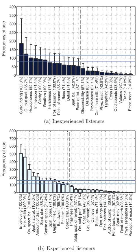
The results of this procedure are shown in Fig. 9, which shows the frequency of use and confidence intervals calcu-lated as described above for each attribute and horizontal lines at the two values ofAsig. For the inexperienced and
ex-perienced listeners respectively, 11 and 15 attributes were used with less than chance frequency. These are the at-tributes to the right of the dashed line in each plot in Fig. 9. For the following analysis, the attributes that were used with less than chance frequency are not shown, with the exception of those that were used by over 70% of partic-ipants (distance, level of reverb, phasiness, and spectral
resonances). Can’t hear difference was excluded as this
was felt to be irrelevant.
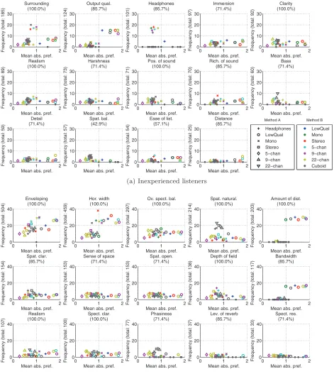
4.3.2 Attribute–Preference Relationship
Fig. 10 shows frequency of attribute use against mean absolute preference for each reproduction method combi-nation, for those attributes that were used by over 70% of participants and/or not used at less than chance frequency (after accounting for discarded values). The points are dif-ferentiated by the two reproduction methods used in each comparison. The plots are ordered by overall frequency of attribute use.
0 50 100 150 200 250 300 350 400 Freq u ency of u se S u rro u nding (100.0%) O u tp u t q u al. (85.7%) Headphones (85.7%) Immersion (71.4%) Clarity (100.0%) Realism (100.0%) Harshness (71.4%)
Pos. of so
u
nd (100.0%)
Rich. of so
u
nd (85.7%)
Bass (71.4%) Detail (71.4%)
Spat.
b
al. (42.9%)
Ease of list. (57.1%)
Discerna
b
ility (57.1%)
Distance (85.7%)
Prominence (57.1%)
Can’t hear diff. (71.4%)
Phys. react. (42.9%) Targetting (42.9%)
Echo (14.3%) Odd so u nds (28.6%) V ol u me (57.1%) Tre b le (14.3%)
Emot. react. (14.3%)
(a) Inexperienced listeners
0 100 200 300 400 500 600 700 800 Freq u ency of u se
Enveloping (100.0%) Hor. width (100.0%)
Ov. spect. b al. (100.0%) Spat. nat u ral. (100.0%) Amo u
nt of dist. (100.0%) Spat. clar. (85.7%)
Sense of space (71.4%)
Spat. open. (71.4%)
Depth of field (100.0%)
Bandwidth (85.7%) Realism (100.0%) Spect. clar. (100.0%) Phasiness (71.4%)
S
ub
j. q
u
al. of rever
b
(57.1%)
Ov. s
ub
j. pref. (57.1%)
Spat.
b
al. (42.9%)
Lev. of rever
b
(85.7%)
Ov. level (57.1%)
Spect. res. (71.4%) Dyn. range (42.9%)
Ens. b alance (14.3%) A u di b
. of comp. (28.6%)
Perc. trans. q
u
al. (57.1%)
Spat. mov. (42.9%)
Real. of rever
b
(28.6%)
Phys. sensation (14.3%) Percept. of noise (14.3%)
[image:11.585.52.289.35.471.2](b) Experienced listeners
Fig. 9. Overall frequency of attribute use for each listener group. Upper and lower horizontal lines show the frequency required for an attribute to be used significantly more or less than chance frequency respectively. Error bars show a proportional distribution of discarded values (see text for full explanation). Dashed vertical lines show the cutoff point of attributes that were used at less than chance frequency after accounting for discarded values. Labels include the percentage of participants that used each attribute.
reproduction method was included in a comparison:
sur-roundingwith the mono reproduction,output qualitywith
the low-quality mono (which also has the largest preference differences), andheadphonesfor the headphone reproduc-tion. The other attributes do not show pronounced relation-ships between frequency of use and preference, tending to be used with approximately equal frequency over the range of preference scores (althoughspatial balance was used mainly for small preference scores, andbassshows an in-crease in frequency for small preference scores). However, some individual comparisons stand out:position of sound
was used most frequently for the mono–cuboid comparison;
richness of soundwas used most frequently for the mono–
stereo comparison;basswas used most frequently for the 22-channel–cuboid comparison; and spatial balance was generally used more for comparisons involving the cuboid. The experienced listener plots show stronger trends. Two attributes were used almost exclusively alongside prefer-ence ratings of a high magnitude (i.e., there is a cluster of points in the top-right corner of the plot), when the low-quality mono speaker was involved in a comparison:
amount of distortionandbandwidth. Other terms were used
more frequently when there was a small difference in pref-erence and less so when there was a pronounced diffpref-erence (most points fall to the left-hand side of the plot):
spa-tial naturalness(particularly for the cuboid reproduction),
depth of field,level of reverb, andspectral resonances. The
remaining attributes were used regardless of the magnitude of preference scores. However,envelopingandhorizontal
widthshow a pronounced trend, being used more frequently
as the preference scores increase.Spatial naturalness,
spa-tial clarity, and phasiness were used more frequently in
comparisons involving the cuboid reproduction method.
4.4 Important Attributes Summary
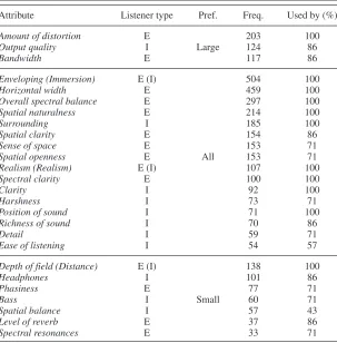
Table 1 gives a summary of the attributes analyzed above, i.e., those that were used at chance frequency or greater as well as those used at less than chance frequency but men-tioned by over 70% of participants. The attributes are sorted by the magnitude of preference judgments for which they were used, then their frequency of use, then the number of participants who gave a response (in the free elicitation stage) that contributed to the attribute. Where an attribute was elicited by both groups of listeners, the inexperienced listeners’ attribute has been indicated in parentheses; Fran-combe et al.[16] found that the experienced listener labels and definitions were preferred by both groups of listeners in cases where the attribute sets overlapped.
5 CONCLUSIONS AND DISCUSSION
A literature review into the attributes that are impor-tant when making preference judgments between spatial audio reproduction methods identified a number of limita-tions of the existing research. Previous studies have been designed to identify all of the differences between listen-ing experiences, rather than just those that make a mean-ingful contribution to listener preference. Similar percepts are often labelled differently across studies, or different percepts are given similar labels. There is a lack of stud-ies in which comparisons between different types of re-production method are drawn, and recent developments in channel-based surround sound with height have not been investigated in detail. The relationship between individual attributes and preference has not been made clear. Finally, inexperienced listeners have not been used in attribute elic-itation studies.
0 1 2 0 10 20 30 Surrounding (100.0%)
Mean abs. pref.
Freq
u
ency (total: 185)
0 1 2
0 10 20 30 Output qual. (85.7%)
Mean abs. pref.
Freq
u
ency (total: 124)
0 1 2
0 10 20 30 Headphones (85.7%)
Mean abs. pref.
Freq
u
ency (total: 101)
0 1 2
0 10 20 30 Immersion (71.4%)
Mean abs. pref.
Freq
u
ency (total: 97)
0 1 2
0 10 20 30 Clarity (100.0%)
Mean abs. pref.
Freq
u
ency (total: 92)
0 1 2
0 10 20 30 Realism (100.0%)
Mean abs. pref.
Freq
u
ency (total: 89)
0 1 2
0 10 20 30 Harshness (71.4%)
Mean abs. pref.
Freq
u
ency (total: 73)
0 1 2
0 10 20 30
Pos. of sound (100.0%)
Mean abs. pref.
Freq
u
ency (total: 71)
0 1 2
0 10 20 30
Rich. of sound (85.7%)
Mean abs. pref.
Freq
u
ency (total: 70)
0 1 2
0 10 20 30 Bass (71.4%)
Mean abs. pref.
Freq
u
ency (total: 60)
0 1 2
0 10 20 30 Detail (71.4%)
Mean abs. pref.
Freq
u
ency (total: 59)
0 1 2
0 10 20 30 Spat. bal. (42.9%)
Mean abs. pref.
Freq
u
ency (total: 57)
0 1 2
0 10 20 30
Ease of list. (57.1%)
Mean abs. pref.
Freq
u
ency (total: 54)
0 1 2
0 10 20 30 Distance (85.7%)
Mean abs. pref.
Freq
u
ency (total: 25)
Headphones LowQual Mono Stereo 5−chan 9−chan 22−chan Method A LowQual Mono Stereo 5−chan 9−chan 22−chan Cuboid Method B
(a) Inexperienced listeners
0 1 2
0 20 40
Enveloping (100.0%)
Mean abs. pref.
Freq
u
ency (total: 504)
0 1 2
0 20 40
Hor. width (100.0%)
Mean abs. pref.
Freq
u
ency (total: 459)
0 1 2
0 20 40
Ov. spect. bal. (100.0%)
Mean abs. pref.
Freq
u
ency (total: 297)
0 1 2
0 20 40
Spat. natural. (100.0%)
Mean abs. pref.
Freq
u
ency (total: 214)
0 1 2
0 20 40
Amount of dist. (100.0%)
Mean abs. pref.
Freq
u
ency (total: 203)
0 1 2
0 20 40
Spat. clar. (85.7%)
Mean abs. pref.
Freq
u
ency (total: 154)
0 1 2
0 20 40
Sense of space (71.4%)
Mean abs. pref.
Freq
u
ency (total: 153)
0 1 2
0 20 40
Spat. open. (71.4%)
Mean abs. pref.
Freq
u
ency (total: 153)
0 1 2
0 20 40
Depth of field (100.0%)
Mean abs. pref.
Freq
u
ency (total: 138)
0 1 2
0 20 40
Bandwidth (85.7%)
Mean abs. pref.
Freq
u
ency (total: 117)
0 1 2
0 20 40
Realism (100.0%)
Mean abs. pref.
Freq
u
ency (total: 107)
0 1 2
0 20 40
Spect. clar. (100.0%)
Mean abs. pref.
Freq
u
ency (total: 100)
0 1 2
0 20 40
Phasiness (71.4%)
Mean abs. pref.
Freq
u
ency (total: 77)
0 1 2
0 20 40
Lev. of reverb (85.7%)
Mean abs. pref.
Freq
u
ency (total: 37)
0 1 2
0 20 40
Spect. res. (71.4%)
Mean abs. pref.
Freq
u
ency (total: 33)
(b) Experienced listeners
Fig. 10. Frequency of attribute use against mean absolute preference for each reproduction method combination. The points are differentiated by the two reproduction methods used in each combination (shape and color). A light gray dot indicates that an attribute was not used for a particular stimulus. The percentage in the title is the percentage of participants that used the attribute.
be used in further evaluations? The conclusions to these questions are discussed below.
5.1 What Spatial Audio Reproduction Methods Do Listeners Prefer?
The Thurstone Case V model was used to produce prefer-ence scales from paired comparison preferprefer-ence ratings for
[image:12.585.54.525.41.568.2]Table 1. Summary of important attributes. The letters “E” and “I” indicate that an attribute was produced by the experienced and inexperienced listeners respectively.
Pref. indicates the approximate magnitude of the mean absolute preference scores most often associated with each attribute. Freq. is the overall frequency of use, and
“used by” indicates the percentage of participants that gave a response that contributed to each attribute.
Attribute Listener type Pref. Freq. Used by (%)
Amount of distortion E 203 100
Output quality I Large 124 86
Bandwidth E 117 86
Enveloping (Immersion) E (I) 504 100
Horizontal width E 459 100
Overall spectral balance E 297 100
Spatial naturalness E 214 100
Surrounding I 185 100
Spatial clarity E 154 86
Sense of space E 153 71
Spatial openness E All 153 71
Realism (Realism) E (I) 107 100
Spectral clarity E 100 100
Clarity I 92 100
Harshness I 73 71
Position of sound I 71 100
Richness of sound I 70 86
Detail I 59 71
Ease of listening I 54 57
Depth of field (Distance) E (I) 138 100
Headphones I 101 86
Phasiness E 77 71
Bass I Small 60 71
Spatial balance I 57 43
Level of reverb E 37 86
Spectral resonances E 33 71
preferred headphone reproduction more than inexperienced listeners, and inexperienced listeners showed a larger pref-erence for the cuboid reproduction. Inexperienced listeners tended to discriminate less between the methods, with little difference between preference for mono and headphones, or between stereo and 22-channel.
It should be noted that this study cannot conclusively state that there may never be a benefit of having more than nine loudspeakers; the systems under test were inextricabil-ity linked with the program material items and the methods used to create them. It is likely that content creators are more practiced at producing program material for lower channel count systems—particularly stereo—and that, as expertise with other systems grows, there may be further benefits available.
5.2 Which Attributes Are Most Important to Listener Experience and Should therefore Be Used in Further Evaluations?
Important attributes were selected by observing which of the attributes were used by the majority of participants and were not used significantly infrequently, as well as by analyzing the relationship between the attribute use and preference scores.
The attributes that were used at chance frequency or greater, as well as those that were used at less than chance frequency but mentioned by over 70% of participants, are summarized in Table 1. The results suggest an approximate hierarchy of attributes. There is a small group of attributes that are consistently associated with large differences in preference between systems; in many regards, these could be considered to be the most important attributes and there-fore should be considered first in evaluation of spatial au-dio systems. These attributes areamount of distortionand
bandwidthfrom the experienced listeners andoutput
qual-ityfrom the inexperienced listeners (although this could be considered to be an umbrella term that includes both as-pects identified by the experienced listeners). However, the pronounced differences in quality associated with these at-tributes are generally produced by the low-quality mono reproduction method; for distinguishing between higher quality methods, different attributes may be more relevant. Other attributes are important regardless of the magnitude of preference; of these attributes,envelopingand
horizon-tal widthwere used very frequently and showed a strong
systems. These attributes aredepth of field,phasiness,level
of reverbandspectral resonancesfor the experienced
lis-teners andheadphones, bass, andspatial balance by the inexperienced listeners.
Some attributes are most frequently used for particular reproduction methods. The experienced listeners mainly
used spatial naturalness and phasiness when describing
comparisons involving the ambisonic cuboid—this is un-surprising given the phase manipulation and small sweet spot involved in first-order ambisonic reproduction. The inexperienced listeners usedsurrounding most frequently in comparisons including the stereo reproduction method,
output quality in comparisons involving the low-quality
mono method,headphones in comparisons involving the headphones, andspatial balancein comparisons including the cuboid.
5.3 Summary
The research presented in this paper was designed to de-termine which reproduction methods listeners prefer and the important attributes that contribute to those preference judgments. It was shown that, broadly, the presence of more spatial content leads to an increase in preference, but that simply adding loudspeaker channels does not necessarily give a corresponding rise in preference. Consequently, the perceptual attributes that contribute to listener preference are of particular interest. Development of perceptually op-timal spatial audio reproduction methods should focus on improving performance on the key attributes.
The results presented above (see Table 1) provide guid-ance to researchers who would like to select attributes for perceptual evaluation of spatial audio reproduction systems. Different attributes might be used depending on the nature of the analysis. For example, a coarse evaluation of low-quality or consumer devices might focus on the attributes that had a large effect on listener preference (amount of
distortion,bandwidth,output quality, and also potentially
envelopmentandhorizontal width, which were commonly
used alongside large differences in preference). Evaluation of high-quality surround sound systems with small differ-ences might focus on more subtle differdiffer-ences (e.g.,depth
of field,phasiness,bass,spatial balance,level of reverb,
andspectral resonances). Finally, where a particular
repro-duction method or facet of the listening experience is under investigation, there might be certain attributes that are of particular interest (e.g.,spatial naturalnessandphasiness
for evaluation of systems including ambisonics).
5.3.1 Future Work
The analysis presented above highlighted some attributes that are important because they contribute significantly to listener preference for spatial audio reproduction methods. The natural progression of this work would be to collect attribute ratings alongside preference ratings for a set of stimuli, which would enable quantitative analysis of each attribute’s contribution to listener preference, as well as validation that the correct attributes were determined to be important.
Determinationofthephysicalparametersthataffect rat-ingsofeachoftheimportantattributesthenleadsnaturally tothedevelopmentofpredictivemodels.Suchmodelscan be used for quick evaluation of existing systems, meter-ing in a spatial audio content production workflow, and developmentofnew,perceptuallyoptimizedspatialaudio reproductionmethods.
6ACKNOWLEDGMENTS
This work was supported by the EPSRC program
Grant S3A: Future Spatial Audio for an Immersive
Listener Experience at Home (EP/L000539/1) and the
BBC as part of the BBC Audio Research
Partner-ship. Details about the data underlying thiswork, along with the terms for data access, are available from https://doi.org/10.15126/surreydata.00809533.
7REFERENCES
[1] ITU-Rrec.BS.2051,“AdvancedSoundSystemfor Programme Production,” Tech. rep.,ITU-R Broadcasing Service(Sound)Series(2014).
[2] J.Francombe,T.Brookes,andR.Mason, “Evalua-tionofSpatialAudioReproductionMethods(Part1): Elic-itationofPerceptualDifferences,”J.Audio.Eng.Soc., vol. 65,pp.198–211(2017Jan./Feb.).
[3]S.ChoiselandF.Wickelmaier,“Extractionof Audi-toryFeaturesandElicitationofAttributesforthe Assess-mentofMultichannelReproducedSound,”J.AudioEng. Soc.,vol.54,pp.815–826(2006Sep.).
[4] S. Choisel and F. Wickelmaier, “Evaluation of
Multichannel Reproduced Sound: Scaling Auditory
Attributes Underlying Listener Preference,” J. Acoust.
Soc. Am., vol. 121, pp. 388–400 (2007),
https://doi.org/10.1121/1.2385043.
[5]N.Zacharov andK.Koivuniemi,“AudioDescriptive Analysis&MappingofSpatialSoundDisplays,”
Proceed-ingsofthe2001InternationalConferenceonAuditory
Dis-play,Espoo,Finland,29July–1August(2001).
[6] H.T.LawlessandH.Heymann,SensoryEvaluation
of Food: Principles and Practices (Springer, New York,
1999),pp.343–346.
[7] F. Rumsey, S. Zieli´nski, R.Kassier, and S. Bech, “OntheRelativeImportanceofSpatialandTimbral Fideli-tiesinJudgmentsofDegradedMultichannelAudio Qual-ity,” J. Acoust. Soc. Am., vol.118, pp. 968–976 (2005), https://doi.org/10.1121/1.1945368.
[8] J. Francombe, T. Brookes, R. Mason, R. Flindt, P. Coleman, Q. Liu, and P. Jackson, “Production and Reproduction of Programme Material for a Variety of Spatial Audio Formats,” presented at the 138th
Con-vention of the Audio Engineering Society (2015 May),
eBrief 199.
[9] E. Parizet, N. Hamzaoui, and G. Sabatie, “Compar-ison of Some Listening Test Methods: A Case Study,”
Acta Acustica united with Acustica, vol. 91, pp. 356–364
[10] R. McGill, J. W. Turkey, and W. A. Larsen, “Vari-ations of Box Plots,”Amer. Statistician, vol. 32, pp. 12–16 (1978), https://doi.org/10.2307/2683468.
[11] E. Parizet, “Paired Comparison Listening Tests and Circular Error Rates,”Acta Acustica united with Acustica, vol. 88, pp. 594–598 (2002).
[12] L. Thurstone, “A Law of Comparative Judg-ment,” Psych. Rev., vol. 34, pp. 273–286 (1927), https://doi.org/10.1037/h0070288.
[13] K. Tsukida, M. Gupta, “How to Analyze Paired Comparison Data,” Tech. Rep. UWEETR-2011-0004, Uni-versity of Washington (2011).
[14] M. G. Kendall and B. Babington Smith, “The Prob-lem ofmRankings,”Annals of Mathematical Statistics, vol. 10, pp. 275–287 (1939).
[15] A. Silzle, S. George, E. A. P. Habets,
and T. Bachmann, “Investigation on the Quality
of 3D Sound Reproduction,” Proceedings of the
First International Conference on Spatial Audio,
Det-mold, Germany, 10–13 November (2011), pp. 334–
341.
[16] J. Francombe, R. Mason, M. Dewhurst, and S. Bech, “Elicitation of Attributes for the Evaluation of Audio-on-Audio Interference,” J. Acoust. Soc. Am., vol. 136, pp. 2630–2641 (2014).
[17] S. Bech and N. Zacharov,Perceptual Audio
Evalu-ation: Theory, Method and Application(Wiley, Chichester,
2006), pp. 186–187.
[18] A. P. Field,Discovering Statistics Using SPSS(Sage Publications, London, 2005), pp. 698–699.
THE AUTHORS
Jon Francombe Tim Brookes Russell Mason James Woodcock
Jon Francombe graduated with a first-class honors de-gree in music and sound recording (Tonmeister) from the University of Surrey, Guildford, UK, in 2010, and received a Ph.D. in perceptual audio quality evaluation from the same institution in 2014. His Ph.D. research investigated the experience of a listener in an audio-on-audio interfer-ence situation. He is currently working as a research fellow on the EPSRC-funded “S3A: Future Spatial Audio” project investigating the perceptual attributes of spatial audio re-production. He has also worked as a music technician, freelance musician, and sound engineer.
•
Tim Brookes received the B.Sc. degree in mathematics and the M.Sc. and D.Phil. degrees in music technology from the University of York, York, UK, in 1990, 1992, and 1997, respectively. He was employed as a software engineer, recording engineer, and research associate be-fore joining, in 1997, the academic staff at the Institute of Sound Recording, University of Surrey, Guildford, UK, where he is now senior lecturer in audio and director of research. His teaching focuses on acoustics and psychoa-coustics and his research is in psychoacoustic engineering: measuring, modeling, and exploiting the relationships
be-tween the physical characteristics of sound and its percep-tion by human listeners.
•
Russell Mason graduated from the University of Sur-rey in 1998 with a B.Mus. in music and sound recording (Tonmeister). He was awarded a Ph.D. in audio engineer-ing and psychoacoustics from the University of Surrey in 2002 and was subsequently employed as a research fellow. He is currently a senior lecturer in the Institute of Sound Recording, University of Surrey, and is program director of the undergraduate Tonmeister program. Russell’s research interests are focused on psychoacoustic engineering includ-ing the development of methods for subjective evaluation and modelling aspects of auditory perception.
•