Outlier labeling via circular boxplot

Outlier labeling via circular boxplot

Abuzaid, A. H.

Hussin, A. G.

Mohamed, I. B.

1_{Institute of Mathematical Sciences, University of Malaya, 50603 Kuala Lumpur, MALAYSIA.}

E-mail: [email protected]

2_{Center for Foundation Studies in Science, University of Malaya, 50603 Kuala Lumpur, MALAYSIA.}

E-mail: [email protected]

3_{Institute of Mathematical Sciences, University of Malaya, 50603 Kuala Lumpur, MALAYSIA.}

E-mail: [email protected]

Keywords: Boxplot, Circular data, Outliers, Overlapping.

Abstract

Boxplot is a simple and flexible graphical tool that has been widely used in exploratory data analysis. Its main application is to identify extreme values and outliers in linear univariate data sets. However, the standard boxplot for linear data set is not suitable to be used for circular data sets due to the bounded property of circular variables. In this paper, we propose and develop a boxplot for circular data sets based on five circular summary statistics which is called circular boxplot. In the process, several problems have been resolved. Firstly, we have overcome the problems of estimating the circular median, the first and second quartiles and overlapping areas between the upper and lower fences. Secondly, we resolve the problem of finding the appropriate boxplot criterion which is (_νIQR=1.5IQR) in linear case, where_IQR is the interquartiles range and _ν is the resistance constant. Through simulation studies, we identify the appropriate values of circular boxplot criterion which depends on the concentration parameter. The power of performances of the proposed boxplot is investigated. We then develop S-Plus subroutines to display the circular boxplot and apply the plot on a real circular data set.

1

Introduction

Visual display is an easy and informative technique to deal with the data. There are various graphs that enable statisticians to present their data such as histogram, pie chart, Q-Q plot and boxplot.

Boxplot is a simple and flexible graphical tool in exploratory data analysis developed by Tukey(1977). It consists of five-number summaries which are the smallest observation, lower quartile_Q1, median, upper quartile _Q3 and largest observation. Its main application is to identify extreme values and outliers in univariate data sets.

Most of text monographs employ 1_.5_IQR boxplot criterion to detect outliers in data sets. In other words, any observation below_Q1−1_.5_IQR or above _Q3+ 1_.5_IQR are labeled as ”outlier”. Extensive research was conducted on the labeling of outlier by using boxplot. Hoaglin et al.(1986) investigated the performance of resistant rules for outlier labeling by using different values instead of_ν = 1_.5. They con-cluded that the main resistant rule_ν = 1_.5 has many advantages especially in avoiding the masking prob-lems. Further, they considered the rule when _ν = 3 as extremely conservative. Ingelfinger et al.(1983) suggested the use of_ν = 2 while Sim et al.(2005) demonstrated that the use of resistant rule_ν = 1_.5 or ν= 3 is in general inappropriate for normal sample and is completely inappropriate for skewed distribu-tions. So the value of_ν differs from data set to another depending on the underlying distribution of the data set.

All known published works on the boxplot were conducted for linear variables. There is no relevant published work on circular variables, except Graedel(1977) who suggested the use of boxplot to improve the wind rose diagram.

There are many phenomena that can be considered as circular variables such as directions of wind and birds immigration. For such data, the linear techniques can no longer be used and special techniques are required as the identification of outliers in circular data requires different approach compared to the linear case. There are several methods available to detect outliers in circular data. Collett(1980) presented four different numerical tests of discordancy in circular data, namely _{C, D, L} statistics and improved _M statistics which was first proposed by Mardia(1975). Abuzaid et al.(2008) identified single

graphical methods.

In this paper the main objectives are to (i) construct a special boxplot for circular data called the circular boxplot (ii) use the circular boxplot in the detection of outliers in circular data and (iii) develop a subroutine in S-Plus environment to draw the circular boxplot.

In the next section we discusses the proposed construction of circular boxplot. Simulation and nu-merical studies are carried out in Sections 3 to estimate the appropriate values of resistance constant_ν. A numerical example is discussed in Section 4 to illustrate the application of circular boxplot in detecting outliers for circular regression based on circular residuals.

2

Summary statistics for constructing circular boxplot

Due to the unusual characteristics of circular variables, many relevant descriptive measures and display plots have been developed for example, circular histogram and stem-and-leaf diagrams. However, there is no known design of boxplot for circular variable. The difficulty of constructing the boxplot for circular variables arises from the complexity of determining the median. This is due to the bounded range of circular variables and the overlapping problem which occurs when the concentration parameter _κ of circular sample is small. These issues will be addressed in this section.

2.1 Median direction of circular variable

Fisher(1993) defined the median of circular variable as an axis which divides the data into two equal groups (median axis). Practically, the circular median is the observation_φ, which minimizes the summa-tion of circular distances, _d(_φ) = _π−n_i=1|_π− |_θi−_φ||. Consistently, Mardia and Jupp(2000) defined the median for a set of circular observations_{θ1, θ2, ..., θn} as any point_φ, where half of the data lie in the arc of [_{φ, φ}+_π) and the other points are nearer to_φthan to_φ+_π. In case of prior knowledge about the circular distribution, Mardia(1972) defined the median direction_φas the solution of

_φ+π

φ f(θ)dθ= _φ+2π

φ+π f(θ)dθ= 0.5.

2.2 Quartiles of circular variables

In order to construct boxplot for circular variable, we need to know the median, the first quartile_Q1 and the third quartile_Q3. Mardia(1972) defined the first and third quartile direction_Q1 and_Q3 as any solution of

_φ

φ−Q1f(θ)dθ= 0.25 and _φ+Q3

φ f(θ)dθ= 0.25,

respectively. In most cases, the circular distribution is unknown. To date, no published literature is found on a nonparametric estimator of _Q1 and _Q3 for circular variables. However, it seems sensible to estimate_Q1 and_Q3 by classifying the sample observations into two groups based on their locations with respect to the sample median direction. Subsequently, _Q1 can be considered as the median of the first group and_Q3 as the median of the second.

Defining_Q1 and _Q3 in such a way may looks trivial because in some cases_Q1 could be larger than Q3. Under this circumstance we can interchange the labels ofQ1 andQ3 due to the compactness and periodicity of the circle. For simplicity and to avoid the confusion caused by the localization of_Q1 and Q3, rotatable property of circular data by subtracting the estimated mean direction of the circular sample from each sample observation is used to make sure that the mean is in the 0 direction. This rotation might be helpful to identify_Q1and_Q3in a more consistent way. Hence, we can assume that_Q1∈(0_{, π}] and_Q3 ∈(_π,2_π). The robustness of mean direction, (see Wehrly and Shine(1981)) is a useful property which gives a fair assurance that the existence of any possible outlier will not have much effect on the estimated mean direction.

IQR= 2_π−_Q3+_Q1.

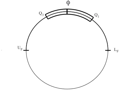
The upper and lower fences can be identified such as, lower fence _LF =_Q1+_νIQR and upper fence UF =Q3−νIQR, where ν is a resistance constant.

After obtaining the median,_{Q1, Q3, LF} and _UF, it is possible to rerotate the sample by adding the estimated mean direction for rotated sample. Figure 1 illustrates the suggested shape of circular boxplot after the rotation. In the following section, numerical and simulation studies will be carried out in order to specify appropriate values of_ν.

.

φ

Q₁ Q3

UF _L

F

Figure 1: The proposed structure of circular boxplot.

3

Estimation of the resistance constant

ν

In linear case, 1_.5_IQRcriterion is a popular method to identify outliers. The interest of investigating the appropriate values of constant _ν was developed since the first construction of boxplot. Researchers like Hoaglin et al.(1986), Ingelfinger et al.(1983) and Sim et al.(2005) discussed the appropriate values of ν which can be used to identify the outlier in linear samples. It is not sensible to utilize similar constants ν of linear boxplot in the case of circular due to the bounded range of the circle. Hence, there is high possibility of overlapping problem between lower and upper fences for large resistance constant _ν when the concentration parameter_κis small.

Hoaglin et al.(1986) used different measures to investigate the behavior of boxplot. In this paper, we employ one of the measurements to estimate an appropriate values of the constant_ν.

3.1 Simulation and numerical studies

In order to investigate the behavior of circular variables with respect to five different summaries which are the median, _{Q1, Q3, LF} and _UF, series of simulation studies are carried out. Samples were generated from von Mises distribution_{V M}(_{µ, κ}) with different sizes between 5 and 200. Different values of concentration parameter _κare considered, _κ = 0_.5_,1(1)10. Further, various values of the resistance constant_ν= 1(0.2)3 and 3.5 are utilized in order to obtain_LF and_UF. The_B(_{ν, n}) denotes the probability that the von Mises sample of size_ncontains no observation outside the interval (_{LF, UF}).

A total of 3000 samples were generated from von Mises distribution _{V M}(_{µ, κ}) for each combination of _nand concentration parameter _κ. The outcomes of simulation studies are _{IQR, Q1, Q3, LF, UF} and B(_{ν, n}).

Let _B(_{ν, n}) denotes the probability of no observation outside the interval (_{LF, UF}) for von Mises sample of size _n and resistance constant _ν. Overlapping problem affects the behavior of _B(_{ν, n}). It is noticed that, for small concentration parameter_κ,_B(_{ν, n}) is non monotone function of _ν, while_B(_{ν, n}) is an increasing function of_ν for large concentration parameter, (_κ≥3). Further, for large concentration parameter (_{κ >}3),_B(_{ν, n}) is not much affected by the increment of _κ, as shown in Figure 2.

1.0 1.5 2.0 2.5 3.0 3.5

ν 0.0

0.2 0.4 0.6 0.8 1.0

k=0.5 k=1 k=2 k=3 k=6 k=10

B(

ν

,

n

)

Figure 2: Behavior of_B(_{ν, n}) measure.

Simulation results of _B(_{ν, n}) are used to specify values of_ν which can be implied on the structure of circular boxplot. It is more informative to interpret the results of simulation studies according to the mod of sample size_nwith respect to 4, the sample size can be clustered into one of 4 groups according to whether_nhas the form 4_j,4_j+ 1_,4_j+ 2 or 4_j+ 3, where_j ∈N.

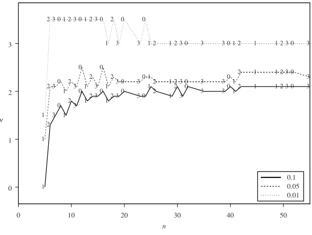
Figure 3 shows the values of_ν for sample size _{n <}56 at 0.1, 0.05 and 0.01 level of significance and large values of _κ, (_κ = 7). It is shown that the values of _ν are decreasing functions of the level of significance. At 0.05 level of significance,_ν values seem to be stationary for (5_{< n <}130), with respect to the remainder after dividing sample size_nby 4. Results suggest that it is appropriate to use the value of resistance constant to be (2_.1_{< v <}2_.7). Simulation results show that the values of_ν increase slightly for larger sample size. Similar behavior can be observed for_α= 0_.1, but the values of resistance constant ν alternate between 1_.5 and 2_.2. The situation is different when_α= 0_.01, where the cut points are fixed at _ν = 3_.5 for (5_{< n <} 25), and decreases to_ν = 3 for larger sample size _n. For small concentration parameter (_{κ <}3), the convenient values of resistance constant_ν are to be less than 2.

4

Numerical example: Wind direction data

0 10 20 30 40 50 n 0 1 2 3 1 2 3 0 1 2 3 0

12 3

0

12 3

0 3 0 1 2 1 2 3 0

3 3012 1 1 2 3 0 3

1

2 30

1 2 3 0 1 2 3 0 1 2

3 0 30 12 1 2 3 0 3 301

2 1 1 2 3 0

3

1

2 3 0 1 2 3 0 1 2 3 0

1 2 3 0 3 0

1 2 1 2 3 0 3 3 0 1 2 1 1 2 3 0 3

0.1 0.05 0.01 ν

Figure 3: Percentile points for different sample size_n, at_κ= 7.

ˆ

yi= 0.165 + 0.973xi(mod2π).

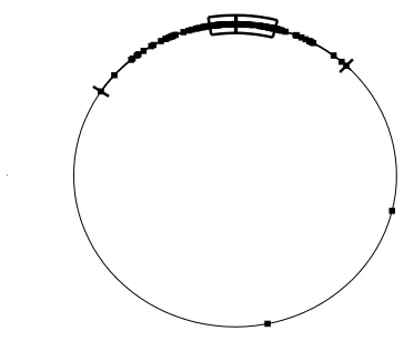
Then the residuals were estimated together with its mean direction (¯_θ= 0_.017), concentration param-eter (ˆ_κ= 7_.34),median direction (_φ = 0_.0072), first quartile (_Q1 = 0_.202), third quartile (_Q3 = 6_.125) and (_IQR= 0_.360). By using numerical and graphical methods, Abuzaid et al.(2008) identified obser-vations number 38 and 111 as outliers. Circular boxplot was used to identify possible outliers in circular regression via the circular residuals. Since ˆ_κ = 7_.34, which is considered large enough, we can use the values of_ν larger than 2.

Table 1 shows the observations detected as an outlier in wind direction data set by using different values of_ν, and the observation numbers 38 and 111 were identified as outliers for all values of_ν.

Table 1: Summary of the observations detected by using several values of_ν for circular residuals of wind data.

ν UF LF Count Observation

1 0.561 5.765 14 15,18,38,43,48,68,70,95,98,99,100,109,111,123. 1.2 0.633 5.693 12 18,38,43,48,68,70,95,98,99,100,111,123. 1.5 0.741 5.586 6 38,43,70,99,100,111.

1.7 0.813 5.514 4 38,43,70,111. 2 0.921 5.406 3 38,43,111. 2.2 1.029 5.298 2 38,111. 2.5 1.101 5.226 2 38,111. 2.7 1.173 5.154 2 38,111. 3 1.281 5.046 2 38,111. 3.5 1.461 4.866 2 38,111.

Figure 4: Circular boxplot of circular residuals of wind data, for_ν=2.5.

5

Conclusions

Boxplot is a popular tool for explanatory data analysis. It was developed gradually over the past 40 years and however there is no known structure of boxplot for circular variables. It is shown that by specifying the median direction, first and third quartiles solve half of the problem of constructing circular boxplot, while the determination of the upper and lower fences are more challengeable because of the bounded rang of the circle. further more the level of concentration parameter is highly affecting the structure of circular boxplot.

There are some interesting points being highlighted based on the simulation studies in Section 3, such as the robustness of mean direction in circular sample and the functional relationship between the_IQR and the large concentration parameter_κ.

It is recommended to use different values of _ν to identify possible outlier in circular variables. For samples with large concentration parameter _κ, it is appropriate to use different values of _ν, where 2 _< ν < 2_.7, while for samples with small concentration parameter _ν, the values of resistant rules can be chosen between 1 and 2. These values are comparable to the linear case in which_ν equal to 1_.5.

Circular boxplot is also able to identify possible outlier in frogs’ data set and the identification results are consistent with Collett(1980).Further, in the case of circular regression model, observation numbers 38 and 111 were identified as outliers by circular boxplot.

We have shown that the circular boxplot can be considered as a new graphical tool for explanatory analysis of circular data, and it is an alternative technique to identify outliers in circular samples and in circular regression through the circular residuals.

References

Abuzaid, A. H., Hussin, A. G. and Mohamed, I. B. (2008). Identifying single outlier in linear circular regression model based on circular distance.Journal of Applied Probability and Statistics, 3(1): 107-117, Dixie W Publishing Corporation.

Barnett, V. and Lewis, T. (1978).Outliers in Statistical Data. New York and London,Wiley.

Collett, D. (1980). Outliers in circular data. Applied Statistics, 29(1): 50-57, Blackwell.

David, H. A. (1970). Order statistics. New York and London, Wiley.

Fisher, N. I. (1993). Statistical analysis of circular data. London, Cambridge University Press.

Hussin, A. G., Fieller N. R. J. and Stillman E. C. (2004). Linear regression for circular variables with application to directional data. Journal of Applied Science and Technology, 8(1 & 2): 1-6, (INSS)and (ICMST).

Ingelfinger, J. A., Mosteller, F., Thibodeau, L. A., and Ware, J. H. (1983). Biostatistics in Clinical Medicine. New York, Macmillan.

Mardia, K. V.(1975). Statistics of directional data.J. R. Statistic. Soc.B, 37: 349-393, Blackwell.

Mardia, K. V. (1972).Statistics of directional data. Academic Press. London.

Mardia, K. V. and Jupp, P. E. (2000).Directional data, 2nd edition. J. Wiley. London.

Sim, C. H., Gan, F. F. and Chang, T. C. (2005). Outlier Labeling With Boxplot Procedures. Journal of the American Statistical Association, 100 (470): 642-652, Alexandria, VA.

Tukey, J. W. (1977).Exploratory data analysis. Addison-Wesley, Reading, MA.