Using Statistical Process Control Charts (SPCC) to Determine Optimum Resolution for Geomorphometric Analyses

Using Statistical Process Control Charts (SPCC) to Determine Optimum Resolution for Geomorphometric Analyses.

by

Nicholas A Nalepa

A thesis submitted in partial fulfillment of the requirements for the degree of

Master of Science (Environmental Science)

in the University of Michigan-Dearborn 2017

Master’s Thesis Committee:

Associate Professor Jacob Napieralski, Chair

ACKNOWLEDGEMENTS

I would like to thank my Mom and Dad. Without their love and support I would not have been

able to finish this thesis. They were very encouraging to pursue my education as far as I could;

farther than I thought was possible. My fiancée Sarah has been very supportive, she has put up

with the stressful days and nights without complaint. Her support has been tremendous, and I

will always love her for it. My family as well my new in-laws have also been very supportive of

me. Their positivity has been uplifting and a good motivator.

I wanted to sincerely thank every member of my Thesis committee. Without you I am not sure

this thesis would have ever happened. Dr. Jacob Napieralski showed me how a class project

could turn into a published paper in a relatively short time with hard work and determination. He

helped me realize my potential and for that I will always be grateful. Through his guidance, I

was able to present at 11 national conferences throughout the USA. It is amazing all the things

you can get out of College if you have great advisor. Dr. Kent Murray introduced me into the

Earth Science program and without that happening, I don’t think I would have ever found a place

where I truly belonged. Dr. Claudia Walters has always supported me and always seemed to be

TABLE OF CONTENTS

ACKNOWLEDGEMENTS ... ii

LIST OF TABLES ... v

LIST OF FIGURES ... vi

ABSTRACT... viii

Chapter 1: Introduction ... 1

Introduction... 1

Digital Surface Representation ... 2

The Impact of Resolution on Geomorphometry ... 3

Determining Optimum Resolution... 4

Drumlin Analysis as Test Case... 5

Thesis Objectives... 6

Thesis Format... 6

References... 9

Chapter 2: The Application of Control Charts to Determine the Effect of Grid Cell Size on Landform Morphometry... 13

Abstract... 13

Introduction... 13

Objective and Scope ... 16

Study Area ... 16

Drumlin Identification and Measurement... 18

Statistical Technique... 21

Results... 23

Basic Drumlin Morphometry... 23

Drumlin Shape ... 26

Drumlin Location... 27

Discussion... 29

General observation and trends... 29

Technique: Boxes... 30

Technique: Statistics ... 31

Future work... 31

Conclusion ... 32

Chapter 3: Optimizing Geomorphology Using Statistical Process Control Methods ... 40

Abstract... 40

Introduction... 41

Statistical Process Control Analysis ... 46

Discussion... 49

Conclusion ... 52

References... 56

Chapter 4: Conclusion... 62

Introduction... 62

Statistical Process Control Charts (SPCC) ... 63

Results... 64

The Impact of Grid Resolution on Geomorphometric Analyses of Drumlins... 64

Optimum Resolution... 64

Measurements ... 64

Limitations to the Use of SPCC... 65

Impact of this Study... 66

Suggestions for Further Research ... 66

LIST OF TABLES

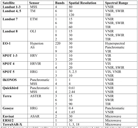
Table 1.1. Summery of available satellite sensors used in landform mapping (A table modified from Napieralski et al, 2013) ...Error! Bookmark not defined.

Table 2.1. Optimum resolutions for each drumlin for each variable. ...Error! Bookmark not defined.

Table 3.1. Summary of drumlin size and optimum DEM resolution for 16 drumlins (in meters). ... 55

Table 3.2. Evaluation of the impact control set size and number of standard deviation has on optimum resolution for width (left) and length (right). ... 55

Table 3.3. Attaining optimum resolution for drumlin area through use of SPCC for each

LIST OF FIGURES

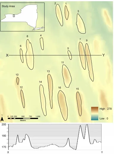
Figure 2.1. Digital elevation model (DEM) of study area, including 16 drumlins analyzed in this study... 17

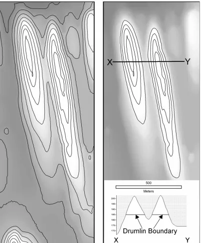
Figure 2.2. Illustration of technique used to identify and extract drumlins using a contoured DEM... 19

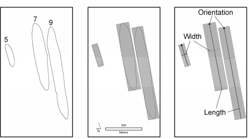
Figure 2.3. Technique used to measure basic drumlin characteristics utilized a series of bounding containers that automatically calculated the width, length, and orientation of each drumlin... 21

Figure 2.4. A conceptual diagram of a control chart used to determine optimum grid cell size for each drumlin... 23

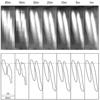
Figure 2.5. Illustration of variations of drumlin shape and size caused by changes in grid cell size ... 24

Figure 2.6. A control chart used to evaluate variations in width of drumlins 2, 11, and 12. UCL and LCL are included in each dataset... 25

Figure 2.7. A summary of optimum resolutions used in this study. This type of summation can be useful when determining optimum resolution with assemblages of drumlins... 27

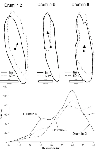
Figure 2.8. As grid cell size increases, a drumlins centroid shifts position, which can be

attributed to a drumlin changing size (drumlin 6), a drumlin physically shifting (drumlins 2 and 8), or a combination of both... 28

Figure 3.1. An extensive summary of previous studies that have analyzed the impact of resolution fall within predictable ranges for grid cell sizes examined and the size of the study area or landform... 43

Figure 3.2. Regional map illustrating prevalence of drumlins in north-central New York, USA (top). Map A presents the drumlins used in this study, including an illustration of individual boundaries for each drumlin and drumlin identification numbers (Map B) ... 45

Figure 3.3. The basic dimensions of a drumlin analyzed in this study. As grid cell size changed, each dimension was re-measured and basic measurements were combined to characterize

Figure 3.4. Illustration of drumlins 14 and 13 delineated from resolutions commonly used in previous and present-day landform studies, including Landsat 1-3, Landsat 5-7, National

Elevation Dataset, and using Light Detection and Ranging ... 48

ABSTRACT

Studying landscapes can give great insight into what geological processes lead to their current

appearance. The use of digital elevation models (DEMs) helps scientists better understand the

processes that created or modified landscapes, especially with study areas that are geographically

extensive. As resolution has increased, scientists have started to notice more subtle details in

features that have not been previously reported in coarser resolution studies. This study’s focus

was on assessing the impact of DEM resolution on the delineation of landforms. There were two

main objectives of this thesis: (1) Determine the optimum resolution for measuring drumlins and

(2) automating the analysis by customizing ArcGIS 9.3 for the morphometric measurements for

use with Statistical Process Control Charts (SPCCs) to determine the optimum resolution of

drumlins. SPCCs are primarily used for process and quality control in manufacturing and

industrial applications. The principles of this method can be applied similarly to the problem of

coarsening of DEM resolution. The problem was treated like an industrial process where the

finest resolutions was treated as the control set, then as resolutions get coarser, a point is reached

where the values exceed acceptable values and are deemed unreliable. The last resolution before

the unreliable value is then deemed the optimum resolution. The study area was in Palmyra, NY,

chosen due to the abundance of drumlins, which are streamlined glacial landforms that are easily

recognizable on contour maps or DEMs. Results indicate that (1) 10 m DEMs were consistently

delineated using a bounding container script. The only task not automated was delineating the

drumlins themselves. This study’s focus was on assessing the impact of DEM resolution on the

delineation of landforms. SPCC helped give statistical significance to optimum resolution rather

than more simplified methods (e.g., inflection point or relative error). All of this combined could

lead to discoveries in landform delineations, patterns, or genesis of not only drumlins, but

Chapter 1: Introduction

Introduction

Resolution is most simply defined as “the process or capability of distinguishing the individual parts of an object”, or “a measure of the sharpness of an image or of the fineness with which a device can produce or record such an image usually expressed as the total number or density of pixels in the image” (Merriam-Webster, 2005). There are four fundamental types of resolution referenced in landform studies (e.g., Shellito, 2012):

• Spatial: the size of the area on the ground being represented by one pixel’s worth of energy measurement.

• Spectral: the bands and wavelengths being measured by a sensor.

• Radiometric: the ability to determine fine differences in a band of energy measurements.

• Temporal: the length of time a sensor takes to come back and image the same location on the ground.

Digital Surface Representation

A digital elevation model (DEM) is a numerical representation of surface elevations over a region of terrain. DEMs provide the same information as contour maps, but in a digital format suitable for processing by computer-based systems rather than in analog format (Cho and Lee, 2002). DEMs can be made by incorporating field observations, stereopairs, topographic maps, or remotely sensed observations (balloon, airplane, satellite, etc.) into a GIS (geographic

information system). DEMs store aggregated ground data for each pixel in raster format. Many DEMs are developed from satellite data, which have gradually decreased in pixel cell size over time. For example, DEMs from early Landsat programs had a resolution of 80 m (i.e., 80 m x 80 m pixels), which produced a relatively coarse representation of Earth’s surface. During the mid to late 1990s, the best available resolution for DEMs was 30 m, which was an improvement in resolution, but still left some ambiguity in accurately measuring a landform, especially if the landform was relatively small (e.g., 40 m wide). In the early 2000s, 10 m DEMs became readily available (Table 1.1), becoming the new standard for high DEM resolution (e.g., the National Elevation Datasets (NED) in the United States, Shellito, 2012). Now users have the ability to study micro-scale landforms, but due to limitations in computing power and storage capacity, many studies are not feasible because of the sheer volume of data and processing time. As technology advances, this gap should lesson to a point where it is negligible. Geomorphologists typically have to decide between studies with larger study areas and coarser resolutions or focusing on subsets of the landscape with finer resolution.

Currently, this technological evolution continues, as Light Detection and Ranging (LiDAR) technology can produce even higher resolution datasets (e.g., sub 1 m). LiDAR has advantages over satellite based data as it is typically gathered with the use of airplanes, which allow

Fourth, vegetation canopies can be easily mapped because there are multiple signals sent; some penetrate the canopy while others can distinguish the top. And lastly, LiDAR can map ground elevations because it penetrates dense vegetation because of multiple signal returns. A

disadvantage is that continuous coverage is not a likely option due to the high costs associated with gathering LiDAR data. Currently, LiDAR data sets are becoming more available to the public due to data being released by private and utility companies.

The Impact of Resolution on Geomorphometry

Many studies have attempted to understand the effects of resolution on landform and landscape characterization derived from DEMs. Clearly, too coarse a DEM resolution decreases the quality of landscape representation, and as a result, delineation and measurement. For example, coarse resolution creates a less defined representation of the landscape (i.e., landscape smoothing), filtering surface roughness and diminishing the accuracy of terrain attributes (Wolock and Price, 1994; Wolock and McCabe, 2000; Thomason et al., 2001; Usery et al., 2004; Claessens et al., 2005; Sorensen and Seibert, 2007; Wise, 2007; Coz et al., 2009; Ely et al., 2016). Additionally, coarse resolution alters slope length and angle, although this is dependent on local topographic variability (Zhang et al., 1999; Thomason et al., 2001; Cotter et al., 2003; Kienzle, 2004; Usery et al., 2004; Paz et al. 2008; Wu et al., 2008; Yu et al., 2015). Finally, the ability to identify and delineate the boundary of a landform (i.e., landform capture) is related to resolution, meaning the total number of landforms identified decreases when resolution decreases (Chaplot et al., 2000; Wu et al., 2008; Yu et al., 2015).

Furthermore, coarse resolution affects hydrologic model simulations of water flow, especially at the watershed scale. Watershed delineation becomes more uncertain when resolution decreases, as coarse resolutions tend to substantially alter watershed shape and size (Cotter et al., 2003). If watershed shape and size are altered, then the derivation of channel networks and flow routing is also impacted (Tang et al., 2003). Resolution also directly influences surface runoff (up to 200% variation) and sediment and nutrient loadings in hydrologic model predictions using

Dixon and Earls, 2012; Tan et al., 2015). Finally, resolution affects estimates of topographic index and soil wetness index (i.e., soil moisture) (Thompson et al., 2000; Wolock and McCabe, 2000; Kienzle 2004; Wu et al., 2008; Tan et al., 2015) and rates of erosion and sedimentation (Schoorl et al., 2000; Woolard and Colby, 2002; Claessens et al., 2005; Hessel, 2005; Hu et al., 2015).

As resolution can have an impact on landscape studies and hydrologic analyses, scientists have sought to determine an “optimum resolution,” which is defined as the coarsest resolution that yields results compairable to finer resolutions (Cotter et al., 2003; Chaplot, 2005; Dixon and Earls, 2009; Yu et al., 2015). Landform characteristics tend to stay relatively similar as resolution is coarsened, but beyond a particular resolution, there is a change in morphometric measurements. A compounding factor is that landforms are also difficult to define because landform boundaries are ambiguous and scientists use different methods to decide what constitutes a boundary. This lack of standardized methods for measuring landforms makes it difficult to compare the results of various landform studies (Dunlop and Clark, 2006; Migon et al., 2013).

Determining Optimum Resolution

To date, the research to determine optimum resolution has been limited. A few studies focused on quantifying the amount of error associated with digital elevation models (Garbrecht and Martz, 1994; Horritt and Bates, 2001; Cotter et al., 2003), and some methods have been as basic as looking for an obvious deviation from the normal pattern or an inflection point on a graph (Horritt and Bates, 2001). Garbrecht and Martz (1994) used the statistical test of relative error in their study, in which they used an arbitrary value of ±10% to determine if resolution is affecting the analysis. These methods were initially tested for this project, but the results were

unsatisfactory and inconsistent in regards to the variety of parameters (area, perimeter, length, width, etc…).

manufacturing processes, but are becoming more common in almost all industries, even finding their way into managing and service orientated occupations (Bissel, 1994). The ability to use SPCCs to monitor short and long-term variability helps maintain a dynamic, changing system. They are designed to make sure products or processes are within specified control limits, which are dictated by a control set within the data. For example, a cereal company would use SPCC for monitoring how much cereal is put into boxes. Too much cereal would result in loss of profits, whereas too little cereal can result in dissatisfied customers. In either case, the use of control limits allows the company to set an acceptable range of product without the risk of losing money or customers.

SPCCs rely on basic statistical principles, including a control set, which is a series of values that are deemed acceptable. Once the control set is determined, the user calculates the amount of variability within the control set (Bissel, 1994). Typically, the analyst uses the amount of variability within the control set to establish a certain amount of standard deviations as control limits. Two to four standard deviations are commonly used, but the boundaries can be flexible if the analyst needs more or less variability to fit their particular needs. These control limits are applied to a base line value, usually the mean value for the control set, resulting in an upper control limit (UCL) and a lower control limit (LCL) that establish action limits. The first time a value exceeds either one, the process is deemed “out of control,” and an action needs to occur to fix the problem. Since control sets are user defined, it is prudent to assess the impact control sets have on the output of the analysis (Napieralski and Nalepa, 2010).

Drumlin Analysis as Test Case

This study was conducted using drumlins as the landform for this DEM analysis. Drumlins are typically used in landform analyses and are easily identified because of their unique shape. They are long, elongated hills found in glaciated areas as a result of previous glacial activity.

distinct shape and distribution throughout the glaciated areas of the USA, Europe, Russia, and China.

Drumlins are of particular interest in this analysis, as they are delineated using the same contour line for each individual drumlin (1m-80m). This clear delineation makes it possible to isolate variations in drumlin measurements that are due to changes in DEM resolution, rather then the algorithm used to delineate the feature.

Thesis Objectives

The scope of this thesis was to first, determine the optimum DEM resolution for measuring drumlins. Second was to develop and modify a statistical test to determine when a resolution is too coarse for landform measurements. The results from this analysis will help guide other studies using SPCC in a DEM analysis of other landforms, possibly varying in magnitude and shape.

Thesis Format

This thesis is formatted in journal paper format, with two of the four chapters written in manuscript form for peer-reviewed scientific professional journals. As a result, there may be some overlap between explanations and discussions between chapters. Because many of these topics relate to one another within the larger objective of the thesis but must be explained in each chapter as they are intended to be stand-alone papers.

The first chapter “Introduction” describes the overall objectives and context of the research, and explains the format of the thesis and how the chapters are related.

range of variables with some being more complex (area, perimeter, elongation) than others (length, width, orientation).

The third chapter, “Optimizing Geomorphometry Using Statistical Process Control Methods” (Napieralski and Nalepa, 2012), was published as a book chapter in Process Control: Problems, Techniques and Applications, written primarily for industrial applications. The methodology focused on the design and application of SPCC and the impact user-defined input variables have on determining an optimum resolution. The results suggest that an optimum resolution does exist for most topographic features.

Satellite Sensor Bands Spatial Resolution Spectral Range

Landsat 1-3 MSS 4 80 VNIR

Landsat 4, 5 TM 6 30 VNIR, SWIR

1 120 TIR

Landsat 7 ETM 1 15 VNIR

6 30 VNIR, SWIR

1 60 TIR

Landsat 8 OLI 1 15 VNIR

8 30 VNIR, SWIR

2 30 TIR

EO-1 Hyperion 220 30 Hyperspectral

Ali 1 10 Panchromatic

9 30 VIR

SPOT 1-3 HRV 1 10 VIR

3 20 VIR

SPOT 4 HRVIR 1 10 VIS

4 20 VNIR, SWIR

SPOT 5 HRG 1 5, 2.5 VIS, VNIR

3 10 VNIR

IKONOS Panchromatic 1 1 VNIR

MSS 4 4 VNIR

Quickbird Panchromatic 1 0.61 VNIR

MSS 4 2.44 VNIR

Terra ASTER 3 15 VNIR

6 30 SWIR

5 90 TIR

Geoeye HRG 1 0.4 Panchromatic

4 1.65 VNIR

Envisat ASAR 2 30 Microwave

ERSI/2 1 30 Microwave

TerraSAR-X 1 1, 3, 18 Microwave

References

Bissel, D. 1994. Statstical Methods for SPC and TQM. Chapman and Hall, New York, 373 pp.

Braun, P., Molnar, T., Kleeberg, H.B. 1997. The problem of scaling in grid-related hydrological process modelling. Hydrological Processes 11, 1219-1230.

Chaplot, V., Walter, C., Curmi, P. 2000. Imporving soil hydromorphy prediction according to DEM resolution and available pedological data. Geoderma 97, 405-422.

Chaplot, V. 2005. Impact of DEM mesh size and soil map scaleon SWAT runoff, sediment, and NO3-N loads predictions. Journal of Hydrology 312, 207-222.

Cho, Sung-Min., Lee, MyungWoo. 2002. Sensitivity considerations when modeling hydrologic processes with digital elevation model. Journal of the American Water Resources Association

37(4), 931-934.

Claessens, L., Heuvelink, G.B.M, Schoorl, J.M., Veldkamp, A. 2005. DEM resolution effects on shallow landslide hazard and soil redistribution modeling. Earth Surface Processes and

Landforms 30, 461-477.

Cotter, A.S., Chaubey, I., Costello, T.A., Soerens, T.S., Nelson, M.A. 2003. Water quality model output uncertainty as affected by spatial resolution of input data. Journal of the American Water Resources Association 39(4), 977-986.

Dixon, B., Earls, J. 2009. Resample or not?! Effects of resolution of DEMs in watershed modeling. Hydrological Processes 23, 1714-1724.

Dixon, B., Earls, J. 2012. Effects of urbanization on streamflow using SWAT with real and simulated meteorological data. Applied Geography 35, 174-190.

Ely, J., Clark, C., Spangolo, M., Strokes, C., Greenwood, S., Hughes, A., Dunlop, P., Hess, D. 2016. Do subglacial bedforms comprise a size and shape continuum? Geomorphology 257, 108-119.

Hessel, R. 2005. Effects of grid cell size and time step length on simulation results of the Limburg soil erosion model (LISEM). Hydrological Processes 19, 3037-3049.

Horritt, M.S., Bates, P.D. 2001. Effects of spatial resolution on a raster based model of flood flow. Journal of Hydrology 253, 239-249.

Hu, W., She, D., Shao, M., Chun, K.P., Si, B. 2015. Effects of initial soil water content and saturation hydraulic conductivity variability on small watershed runoff simulation using LISEM.

Hydroloogical Sciences Journal 60(6), 1137-1154.

Kienzle, S. 2004. The Effect of DEM Raster Resolution on First Order, Second Order, and Compound Terrain Derivatives. Transactions in GIS 8(1), 83-111.

Le Coz, M., Delclaux, F., Genthon, P., Favreau, G. 2009. Assessment of Digital Elevation Model (DEM) aggregation methods for hydrological modeling: Lake Chad basin, Africa. Computers and Geosciences 35, 1661-1670.

Meng, X., Currit., Zhao, K. 2010. Ground Filtering Algorithms for Airborne LiDAR Data: A Review of Critical Issues. Remote Sensing (2), 833-860.

Merriam-Webster, Incorporated. 2005. RR Donnelley, Springfield MA, 425.

Migon, P., Kasprzak, M., Traczyk, A. 2013. How high-resolution DEM based on airborne LiDAR helped to reinterpret landforms – examples from the Sudetes, SW Poland. Landform Analysis 22, 89-101.

Miller, Jesse W. Jr. 1972. Variations in New York Drumlins. Annals of the Association of American Geographers 62(3), 418-423.

Napieralski, J., Barr, I., Kamp, U., Kervyn, M., 2013. Remote Sensing and GIScience in

Geomorphological Mapping. In: Shroder J. (ed), Bishop M.P., Treatise on Geomorphology. Vol. 3. Remote Sensing and GIScience in Geomorphology. Academic Press, San Diego: 187-227.

Napieralski, J., Nalepa, N. 2012. Optimizing geomorphometry using statistical process control methods. In: Werther, S.P. (ed) Process Control: Problems, Techniques, and Applications, 111-125.

Paz, A.R., Collischonn, W., Risso, A., Mendes, C.A.B. 2008. Errors in river lengths derived from raster digital elevation models. Computers and Geosciences 34, 1584-1596.

Schoorl, J.M., Sonneveld, M.P.W., Veldkamp, A. 2000. Three-dimensional landscape process modeling: The effect of DEM resolution. Earth Surface Processes and Landforms 25, 1025-1034.

Shellito, B.A. 2012. Introduction to Geospatial Technologies. W.H. Freeman and Company, New York, 469 pp.

Sorensen, R., Seibert, J. 2007. Effects of DEM resolution on the calculation of topographical indices: TWI and its components. Journal of Hydrology 347, 79-89.

Tan, M.L., Ficklin, D.L., Dixon, B., Ibraham, A.L., Yusop, Z., Chaplot, C. 2015. Impacts of DEM resolution, source, and resampling technique on SWAT-simulated streamflow. Applied Geography 63, 357-368.

Tang, G., Hui, Y., Strobl, J., Liu, W. 2001. The impact of resolution on the accuracy of hydrologic data derived from DEMs. Journal of Geographical Sciences 11(4), 393-401.

Thompson, J.A., Bell, J.C., Butler, C.A. 2001. Digital elevation model resolution: effects on terrain attribute calculation and quantitative soil-landscape modeling. Geoderma 100, 67-89.

Usery, E.L., Finn, M.P., Scheidt, D.J., Ruhl, S., Beard, T., Bearden, M. 2004. Geospatial data resampling and resolution effects on watershed modeling: A case study using the agricultural non-point source pollution model. Journal of Geographical Systems 6, 289-306.

Valeo, C., Moin, S.M.A. 2000. Grid-resolution effects on a model for integrating urban and rural areas. Hydrological Processes 14, 2505-2525.

Wolock, D., Price, C. 1994. Effects of digital elevation model map scale and data resolution on a topography-based watershed model. Water Resources Research 30(11), 3041–3052.

Wolock, D.M., McCabe, G.J. 2000. Differences in topographic characteristics computed from 100- and 1000-m resolution digital elevation model data. Hydrological Processes 14, 987-1002.

Woolard, J.W., Colby, J.D. 2002. Spatial characterization, resolution, and volumetric change of coastal dunes using airborne LIDAR: Cape Hatteras, North Carolina. Geomorphology 48, 269-287.

Wu, S., Li, J., Huang, G.H. 2008. A study on DEM-derived primary topographic attributes for hydrologic applications: Sensitivity to elevation data resolution. Applied Geography 28, 210-233.

Wu, W., Fan, Y., Wang, Y., Liu, H. 2008. Assessing effects of digital elevation model resolutions on soil-landscape correlations in a hilly area. Agriculture, Ecosystems and Environment 126, 209-216.

Yu, P., Eyles, N., Sookhan, S. 2015. Automated drumlin shape and volume estimation usuing high resolution LiDAR imagery (Curvature Based Relief Separation): A test from the Wadena Drumlin Field, Minnesota. Geomorphology 246, 589-601.

Chapter 2: The Application of Control Charts to Determine the

Effect of Grid Cell Size on Landform Morphometry

Abstract

Geoscientists have become increasingly dependent on digital elevation models (DEMs) to delineate and measure landforms and landscapes. However, the DEM grid cell size available may not be the optimum resolution; this can mask subtle changes in measurements and lead to erroneous results. This paper presents a standardized statistical technique (i.e. statistical process control charts (SPCC)) for determining the optimum DEM resolution (i.e. the coarsest resolution in which detail is not sacrificed) for landforms (e.g. drumlins). For this study, forty-four DEM resolutions, ranging from 1 m to 80 m, were used to assess the effect of resolution on drumlin size, shape, and centroid. The results indicate that the optimum resolution for the size variables (width and length) was coarser than the optimum resolution for shape indices (elongation and rose curve). Drumlin location tends to drift in a predictable direction and rate as grid cell size coarsens above particular thresholds. The results prove that resolution plays a critical role in correctly evaluating drumlin morphometry and that care must be taken when utilizing DEMs to summarize drumlin characteristics. The creation of a standardized technique to describe drumlins will allow for scrutiny of previous work and straightforward comparative analyses between studies, while utilizing the optimum resolution will help decipher landform patterns, reveal relationships, and provide more insight into landform evolution.

Introduction

landforms (e.g. drumlins), reveal previously unrecognized relationships between landforms (e.g. ribbed moraines), and support or refute hypotheses for landform and landscape genesis and development. For example, glacial geomorphologists have long debated the environmental conditions under which ribbed moraines form (see Dunlop and Clark, 2006 for summary), with the lack of consensus driven in part by inconsistent descriptions and compilations of shapes and sizes documented from relatively localized studies. Dunlop and Clark (2006) addressed this issue by combining satellite imagery with DEMs to measure and compare the size, shape, pattern, and distribution of ribbed moraines formed by the Scandinavian, Laurentide, and Irish Ice Sheets. The results indicated that held assumptions regarding their formation were inaccurate or untrue, and that the morphological characteristics were more complex than previous studies had

described. Therefore, DEMs promote opportunities to conduct large scale studies (greater than 50,000 km2) of landforms in a rigorous, quantitative manner within a geographic information system (GIS), while also providing a tool that can supplement field mapping and interpretations from aerial photographs.

Napieralski et al., 2007). Therefore, detailed morphometric and pattern analyses of drumlins and drumlin fields enhance reconstructions of paleo-environments.

Although drumlins are well documented and studied, the techniques used to identify, measure, and characterize drumlins have varied with very little consistency. Early methods used

topographic maps to delineate and quantify drumlins on the basis of the enclosed contour line method. Miller (1972) utilized a contour interval of 6.1 m to characterize drumlin form while Trenhaile (1975) identified drumlins using 1:50,000 maps with a contour interval of 8.1 m, supplemented by the use of aerial photographs, to decipher smaller drumlins. It is likely that the use of these intervals was more of convenience, limited by the interval of the topographic maps. Rose (1989) used triangulation, precise leveling and plane tabling to create elevation data at a scale of 1:500 with a contour interval of 0.5 m. However, DEMs and aerial imagery now provide more flexibility with selecting appropriate contour intervals and resolutions to conduct a drumlin analysis (e.g. Kerr and Eyles 2007; Lanier and Norton, 2003; Smith and Wise, 2007). Many of the original drumlin studies required extensive field mapping or tedious plotting from

topographic maps, but DEMs and GIS can be used to develop a drumlin delineation technique that is suitable for various geomorphmetric/physiographic conditions. Multi-resolution DEMs are useful in the accuracy assessment of delineated drumlins according to the differences quantified in drumlin parametric representation.

Despite the extensive history of drumlin descriptions and the resulting variability in drumlin analysis techniques, few studies have assessed how the results of drumlin morphometric studies are influenced by variations in grid cell size when analyzing drumlins on a DEM by employing the enclosed contour technique. Intuitively, relatively fine DEM resolutions resolve more detail and provide more reliable measurements (Gao, 1995; 1997; Ziadat, 2007). Ziadat (2007) found that the accuracy of landscape representation decreases as grid cell size increases. This

found that increasing resolution from 30 m to 15 m increased the count of drumlins by 170%, indicating that coarse resolutions can obscure smaller landforms.

An increase in resolution, however, does not necessarily equate to an increase in detail or detectable landforms especially when far below the typical landform size; rather, very fine resolutions may simply produce more data and increase processing time without improving the quality of the analysis. Therefore, the coarsest resolution in which there is a negligible sacrifice in detail is an optimum resolution to conduct terrain analyses, particularly those related to drumlins.

Objective and Scope

The key objectives of this study are to: 1) present a method for drumlin delineation and

parametric representation from multi-resolution DEMs and 2) determine the influence of DEM spatial resolution on the calculation of drumlin size, shape, and location. Changes in the basic morphometric variables (width, length, and orientation), shape indices (elongation and the rose curve), and location of drumlin center are all evaluated as the DEM grid cell size is altered. Optimum DEM resolution is defined as the resolution for which the pixel size influences calculations of drumlin variables.

Study Area

Figure 2.1. Digital elevation model (DEM) of study area, including 16 drumlins analyzed in this study. A vertical profile from X to Y illustrates the topographic characteristics and reveals a combination of subtle, low-relief drumlins and distinct, high-relief drumlins.

Drumlin Identification and Measurement

A 1 m DEM was generated from the Palmyra topographic map by digitizing the contour lines and interpolating a surface using ArcMap. This 1 m DEM was then sub-sampled to generate DEMs of 2 – 35 m (in increments of 1 m) and 35 – 80 m (in increments of 5 m). Digital contours with an interval equal to 1 m were derived from each sub-sampled DEM. A drumlin was

Figure 2.2. Illustration of technique (at least three enclosed contour lines) used to identify and extract drumlins using a contoured DEM. Note a vertical profile showing relief of the drumlins and where lowest enclosed contour line (5 m interval) is positioned on DEM.

Drumlin length, width, and orientation were calculated for each drumlin by generating a “bounding container” around each drumlin. A bounding container script was developed (and is available from http://arcscripts.esri.com/details.asp?dbid=14535) so that a rectangle was

up” the features by deleting unused contour lines. This study’s only contour lines of interest were the lowest enclosed contour lines which delineated the extent of each drumlin. The boundary of the container box is tangential to each side of a drumlin, such that the width, length, and

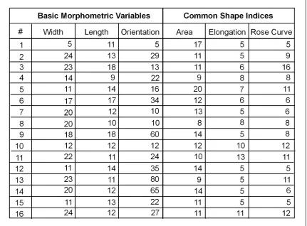
orientation of the box represent the width, length, and orientation of the drumlin (Fig. 2.3). Elongation, area, and the rose curve were also calculated. Elongation is calculated using length/width, while area is simply length×width. The rose curve, which has been found to be a good description of drumlin form (Doornkamp and King, 1971), is defined by the following equation:

R = a cos k

where a is the long axis length and k is a dimensionless constant that defines the elongation of a loop (Chorley, 1959), such that:

k = a2/4A

Figure 2.3. Technique used to measure basic drumlin characteristics utilized a series of bounding containers that automatically calculated the width, length, and orientation of each drumlin.

Finally, the influence of grid cell size on the spatial location of drumlins was investigated by generating a centroid per drumlin at every sub-sampled resolution. The “drift” (i.e. relative movement of the centroid) and drift direction was analyzed because we expect grid cell size to also effect spatial pattern analyses (e.g. cluster analyses), which provide data on the spatial distribution of drumlins and relationships and correlations between drumlins and

surface/subsurface variables.

Statistical Technique

considered unknown, we assume the finest DEM (1 m) generates the most accurate

representation of the landscape and that the reliability of the measurements decrease as the resolution coarsens.

Control charts include two key variables: a range and a set of control limits (upper and lower). The range (R) is calculated from a control set for each drumlin, which in this case is based on the first five resolutions (1–5 m):

R = max – min

where max and min are the maximum and minimum values within the control set (Fig. 2.4). The mean (Ū) range values for the sixteen drumlins were used establish an upper and lower control limit based on a standard deviation (σ):

σ = Ū/1.023

Upper and lower control limits, commonly referred to as action lines, are defined by ±4σ and added to the mean variability within the control set for each drumlin. The first measurement that falls outside the upper control limit (UCL) or lower control limit (LCL) is considered

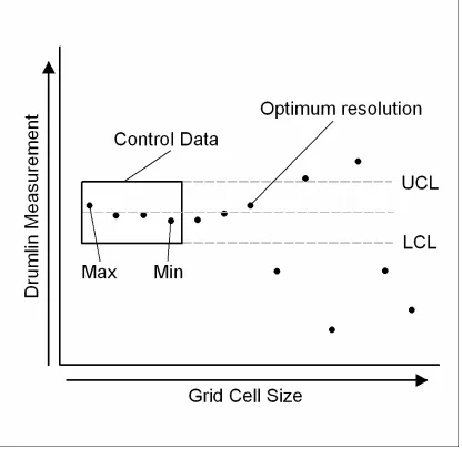
Figure 2.4. A conceptual diagram of a control chart used to determine optimum grid cell size for each drumlin. An upper and lower control limit (UCL and LCL) is calculated from minimum and maximum (range) values found within a control set of each drumlin. Last measurement (e.g. width, length) that falls within the UCL and LCL is considered optimum resolution.

Results

Basic Drumlin Morphometry

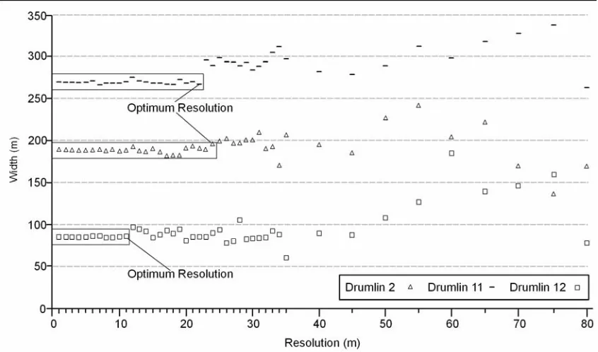
between drumlin width and the optimum resolution is found, as the smallest widths produced the smallest optimum resolutions. Drumlins 5, 10, and 12 had the three smallest widths and smallest optimum resolution (with the exception of drumlin 1). This wide range of widths was common for all drumlins throughout the study area. In particular, drumlin 12 exhibited little variability between resolutions 1-11 m; however, after 11 m, width calculations began to fluctuate between a high value of 186 m and a low calculation of 57 m (a range of 129 m for a drumlin that

measures 84 m across) (Fig. 2.6).

Figure 2.6. A control chart used to evaluate variations in width of drumlins 2, 11, and 12. UCL and LCL are included in each dataset. Optimum resolution for drumlins 2, 11, and 12 is 24, 22, and 11 (see Table 1). Note variability in width calculations with resolutions larger than optimum resolution.

Drumlin length within the study area ranged between 244 – 1279 m (as determined from a 1 m DEM). Surprisingly, calculations of drumlin length were more sensitive to resolution than width or orientation. Initially, we believed that drumlin width was the “limiting variable” because it is the smallest dimension, at times less than 100 m. However, the length of drumlins was frequently affected by substantial portions of the drumlin being removed, which also tended to influence the drift of the drumlin centroid (see below for drumlin location). In most cases, the changes in length caused by increases in grid cell size behaved similarly to width, having little variability between 1-10 m and significant variability with coarser resolutions (equal to or larger than the optimum resolution).

optimum orientation resolution of 60 m but an optimum width and length resolution of 18 m. Therefore, as resolution increased beyond 18 m, the drumlin size changed without rotating.

Overall, the average optimum resolution for the sixteen drumlins was 17 m (width), 13 m

(length), and 29 m (orientation). For most drumlins, the measurements of each variable remained constant as resolution increased from 1 m to 10 m, indicating that a 10 m DEM would be as effective as any sub-10 m DEM when analyzing drumlin characteristics.

Drumlin Shape

Elongation, area, and the rose curve were more sensitive to changes in grid cell size than the

basic variables (see Fig. 2.7). Because each of these indices relied on at least two of the basic

variables, the sensitivity to changes in resolution was exacerbated. As a result, two important

trends differentiated shape indices from the basic variables. First, the range used to calculate the

UCL and LCL for elongation, rose curve, and area were smaller than the range values for width,

length, and orientation, which causes tighter control limits. Second, tight control limits results in

finer optimum resolutions and as a result, most drumlins had an optimum resolution of less than

10 m for the three indices. Exceptions to this trend include drumlins 10, 11, and 16, which also

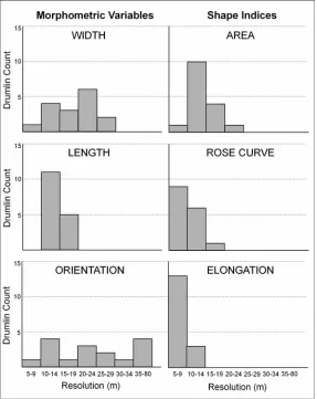
Figure 2.7. A summary of optimum resolutions used in this study. This type of summation can be useful when determining optimum resolution with assemblages of drumlins (drumlin fields). Shape indices are more sensitive to changes in resolution than basic variables, but as a general rule, conducting a drumlin study at resolutions of 30 m or greater will not produce more reliable results.

Drumlin Location

increase in grid cell size and the generalization of bounding contours, the lowest enclosed contour appear at a lower elevation, typically north of the original drumlin location.

Discussion

General observation and trends

Results from this case study indicate that grid cell size clearly influences the measurements and descriptions of drumlin characteristics. The amount of influence occurs at different grid cell sizes for each drumlin and there is no visible trend that indicates which resolution generates unreliable measurements of drumlin characteristics. However, as a general rule, the optimum resolution for calculating drumlin width, length, and orientation ranged between 10-30 m. Although the

optimum resolution for one drumlin may not be the same for another, the 10 m DEM

consistently registered as an acceptable resolution for reliable morphometric studies of drumlin fields. Drumlin fields that contain unusually small drumlinized features, such as in the Tweed basin, Scotland, may require customizing by spatially analyzing subsections of the drumlin field with a high number of small features or using a finer resolution. Furthermore, 10 m elevation datasets are becoming readily available (e.g. NED) and can be used in regional studies without requiring significant processing capabilities. Based on the results of this study, it is not

recommended to use a DEM resolution of 30 m, since almost all drumlins exhibit drastic change in size with resolutions coarser than 30 m.

A coarse optimum resolution could be caused by: 1) substantial variability within the control data (unusually large offset between the minimum and maximum data values within the control group, see Fig. 2.4), or 2) very little change in drumlin size and shape, such that the

While contour interval is not discussed at length in this paper, the interval used to extract drumlins is important. Figure 2.2 illustrates the method of delineating and extracting a drumlin based on a 5 m contour interval. The vertical profile of the drumlin shows where the lowest enclosed contour line exists (185 m). Based on the vertical profile, however, one could argue the base of the drumlin is located near the trough between the two drumlins (181 m), which is actually concealed by a 5 m contour interval. Thus, the next lowest contour line (180 m) is shared by both drumlins and, for the purpose of this study, is removed. This will undoubtedly influence the size and shape of a drumlin. Certainly, the base height that drumlins are derived from can be altered to address this issue but in most drumlinized landscapes, there is a general dip (here, towards the north) that is difficult to account for with most GIS contouring toolboxes.

While 1 m contour intervals were consistently used in this study to provide the most detail and isolate grid cell size as the variable of interest, most DEMs will have at least a few meters of uncertainty, whether derived from satellite imagery, topographic maps, or aerial

photogrammetry. Dunlop and Clark (2006) reported vertical accuracies of ±10 m for ASTER derived DEMs and ±2.5-5.0 m for DEMs derived from aerial photogrammetry. In addition, the horizontal accuracy of contour lines (if derived from a DEM) is a function of the vertical and linear error of the DEM and should be considered when using control charts to determine optimum resolution. In many landform studies, field observations can be used to determine the base elevation of a particular landform, thus minimizing dependence on digital data to derive landform boundaries.

Technique: Boxes

used to provide consistency in this process throughout the drumlin identification and extraction process.

Technique: Statistics

While there are many variations of SPCC, we used upper and lower control limits to indicate when the measurement of a drumlin variable began to vary statistically and, as a result, decrease in reliability. We used the first five resolutions of every drumlin to calculate the standard

deviation because the values were generally consistent within this range for all drumlins; these measurements were used to provide the limits for acceptability for calculations of each drumlin variable. Rather than statistically analyzing each drumlin as a discrete object, the mean standard deviation of the drumlin field (here, 16 drumlins) was used to generate the UCL and LCL for each drumlin. This was done to allow some flexibility in the analyses, as some drumlins showed no measurement variability within the first five resolutions, while other showed subtle variations. The end product of this difference is that some drumlins would have tighter UCL and LCL than others, even though the drumlin sizes and shapes varied equally. However, drumlin fields with enormous variations in drumlin dimensions may be influenced by the use of a mean standard deviation and, as a result, we recommend conducting a sensitive analysis beforehand to determine if the mean or individual standard deviation is favorable for determining optimum resolution.

Future work

Applying this technique to a larger study area would yield more insight into the effectiveness of the bounding container method and the reliability of the statistical analysis used to describe drumlin form. However, the data management obstacle associated with the large amount of digital data required for building 1 m DEMs covering extensive regions would remain, although results from this study suggest that using a DEM less than 10 m (i.e. NED) would be

unproductive and time consuming.

sensitive to changes in resolution, including forms of circularity and comparison measurements (Chan and So, 2006; Maceahren, 1985; Miller and Wentz, 2003; Taylor, 1971). Several of these indices have recently been used as surrogates for elongation (MacLachlan and Eyles, 2007; Nalepa and Napieralski, 2007) and a good correlation between elongation and circularity when measuring drumlin shape has been found (Nalepa and Napieralski, 2007). As different indicators of shape are merged into drumlin studies, it is recommended that the influence grid cell size has on each of these indices is taken into consideration.

Since many studies have utilized contrasting techniques for identifying and measuring drumlins, it may be worthwhile to re-evaluate these results by utilizing the optimum resolution to conduct comprehensive studies of drumlin form and patterns. Additionally, recent studies have focused on the impact of grid cell size variation on hydrologic models, such as the United States

Department of Agriculture’s Soil and Water Assessment Tool (SWAT), watershed delineations, and slope form definition (Alarcon et al., 2006; Chaubey et al., 2005; Gao, 1997; Hutchinson and Gallant, 2000; Marcus et al., 2004; Martz and Garbrecht, 1992; Thieken et al., 1999; Yin and Wang, 1999; Zhang and Montgomery, 1994), creating applications of this technique beyond drumlins.

Conclusion

We developed a semi-automated technique for the identification, extraction, and measurement of drumlins using GIS. Bounding containers quickly and effectively measured the dimensions of drumlins, reducing the subjectivity of drumlin analyses and also increasing the efficiency of what was traditionally a laborious task. In addition, this technique was used to determine the influence DEM grid cell size has on calculations of drumlin variables. The measurements of sixteen drumlins using a range of DEM resolutions demonstrated that grid cell size plays an important role in characterizing drumlin form and, with the use of Statistical Process Control Charts, determined the optimum resolutions that best characterize drumlin form without the use of excessively fine DEM resolutions (increased processing time and storage). The results from this study indicated that a 10 m DEM (e.g. NED) produced calculations of length, width, and

References

Alarcon, V. J., O’Hara, C. G., McAnally, W., Martin, J., Diaz, J., Duan, Z. 2006. Influence of elevation dataset on watershed delineation of three catchments in Mississippi. Geographic Information Systems and Water Resources IV, American Water Resources Association (AWRA), Houston, TX, May 8-10.

Augustin, J.-C., Brice Minvielle, B. 2008. Design of control charts to monitor the microbiological contamination of pork meat cuts. Food Control 19, 1, 82-97.

Bissel, D. 1994. Statstical Methods for SPC and TQM. Chapman and Hall, New York, 373 pp.

Boulton, G. S., Clark, C. D. 1990. A highly mobile Laurentide Ice Sheet revealed by satellite images of glacial lineations. Nature 346, 813-817.

Boyce, J. J., Eyles, N. 2000. Architectural element analysis applied to glacial deposits: internal geometry of a late Pleistocene till sheet, Ontario, Canada. Geological Society of America Bulletin

112, 98-118.

Briner, J. 2005. Do long subglacial bedforms indicate fast ice flow? – A case study from New York. Geological Society of America Abstract with Programs, Northeastern Section, 37, No. 1, p. 22.

Chan, A. H. S., So, D. K. T. 2006. Measurement and quantification of visual lobe shape characteristics. International Journal of Industrial Ergonomics 36, 541-552.

Chaubey, I., Cotter, A. S., Costello, T. A., Soerens, T. S. 2005. Effect of DEM data resolution on SWAT output uncertainty. Hydrologic Processes 19, 621-628.

Chorley, R. J. 1959. The shape of drumlins. Journal of Glaciology 3, 339–44.

Clark, C. D., Wilson, C. 1994. Spatial analysis of lineaments. Computers & Geosciences 20, 1237-1258.

Doornkamp, J. C., King, C. A. M. 1971. Numerical Analysis in Geomorphology. Edward Arnold, London, 608 pp.

Dongelmans, P. 1996. Glacial dynamics of the Fennoscandian ice sheet: a remote sensing study. Unpublished Ph.D. Thesis. University of Edinburgh University, U.K, 245 pp.

Dunlop, P., Clark, C. D. 2006. The morphological characteristics of ribbed moraine. Quaternary Science Reviews 25, 1668-1691.

Ebers, E. 1926. Die bisherigen ergebnisse der drumlin-forschung. Eine monographie der drumlins. (Results of previous drumlin research. A monograph on drumlins.) Neues Jahrbuch fuer Mineralogie, Geologie und Palaeontolgie. 53B, 153-270.

Ebers, E. 1937. Zur entstehung de drumlins als stromlinien körper. (The genesis of drumlins as aerodynamic features.) Neues Jahrbuch fuer Mineralogie, Geologie und Palaeontolgie. 78B, 200-239.

Gao, J. 1995. Comparison of sampling schemes in constructing DTMs from topographic maps.

ITC Journal 1, 18-22.

Gao, J. 1997. Resolution and accuracy of terrain representation by grid DEMs at a micro-scale.

International Journal of Geographical Information Science 11, 199-212.

Gardiner, V. 1983. The relevance of geomorphometry to studies of Quaternary morphogenesis. In: Briggs, D. J., Waters, R. S. (Eds.). Studies in Quaternary Geomorphology: Proceedings of the VIth British-Polish Seminar (International symposia series), Geo Books, Norwich, England, pp 1- 17.

Hutchinson, M. F., Gallant, J. C. 2000. Digital elevation models and representation of terrain shape. In: Wilson, J. P., Gallant, J. C. (Eds). Terrain Analysis: Principles and Applications. John Wiley & Sons, Hobokem, New Jersey, pp. 29-50.

Kerr, M., Eyles, N. 2007. Origin of drumlins on the floor of Lake Ontario and in upper New York State. Sedimentary Geology 193, 7-20.

Kleman, J., Hättestrand, C., Borgström, I., Stroeven, A. 1997. Fennoscandian palaeoglaciology reconstructed using a glacial geological inversion model. Journal of Glaciology 43, 283-299.

Kleman, J., Hättestrand, C., Stroeven, A. P., Jansson, K. N., De Anglis, H., Borgström, I. 2006.

Reconstruction of palaeo-ice sheets- inversion of their glacial geomorphological record. In: Knight, P. (Ed.), Glacier Science and Environmental Change, Blackwell Publishing, pp. 192-198.

Kolesar, P. J. 1993. The relevance of research on statistical process control to the total quality movement. Journal of Engineering and Technology Management 10(4), 317-338.

Lanier, A. J., Norton, K. P. 2003. GIS based analysis f the Chautauqua drumlin field, northwest Pennsylvania and Western New York, Geological Society of America Annual Meeting, Seattle, Washington, Paper No. 188-29.

Li, Y., Napieralski, J., Harbor, J., Hubbard, A. 2007. Identifying patterns of correspondence between modeled flow directions and field evidence: An automated flow direction analysis.

Computers & Geosciences 33, 141-150.

Lopez, C. 2000. Improving the elevation accuracy of digital elevation models: A comparison of some error detection procedures. Transactions in GIS 4, 43-64.

Maceachren, A. M. 1985. Compactness of geographic shape: Comparison and evaluation of measures. Geografiska Annaler 67 B, 53-67.

MacLachlan, J. C., Eyles, C. H. 2007. A quantitative solution to the drumlin debate? Geological Survey of America Annual Meeting, Denver, CO Paper No. 53-34.

Marcus, W. A., Aspinall, R. J., Marston, R. 2004. Geographic information systems and surface hydrology in mountains. In: Bishop, M. P., Shroder, Jr., J. F (Eds.), Geographic Information Science and Mountain Geomorphology. Springer-Verlag, New York, pp. 343-380.

Martz, L. W., Garbrecht, J. 1992. Numerical definition of drainage network and subcatchment areas from digital elevation models. Earth Surface Processes and Landforms 18, 747-761.

Menzies, J. 1984. Drumlins: A Bibliography, Geo Books, Norwich. 117 pp.

Menzies, J., Rose, J. (Eds.), 1987. Drumlin Symposium: Proceedings of the Drumlin Symposium, First International Conference on Geomorphology, Manchester, 1985, A.A. Balkema, Rotterdam & Boston, 360 pp.

Menzies, J., Zaniewski, K., Dreger, D. 1997. Evidence from microstructures of deformable bed conditions within the drumlin at Chimney Bluffs, New York State. Sedimentary Geology 111, 161-171.

Miller, H. J., Wentz, E. A. 2003. Representation and spatial analysis in Geographic Information Systems. Annals of the Association of American Geographers 93(3), 574-594.

Nalepa, N., Napieralski, J. 2007. Comparing the reliability of different compactness and shape indices to measure drumlin form. East Lakes Division Association of American Geographers Regional Meeting, Lansing, MI, October 19-20.

Napieralski, J. 2007. GIS and field-based spatio-temporal analysis for evaluation of paleo-ice sheet simulations. The Professional Geographer 59, 173-183.

Napieralski, J., Hubbard, A., Li, Y., Harbor, J., Stroeven, A. P., Kleman, J., Alm, G., Jansson, K. 2007. Towards a GIS assessment of numerical ice-sheet model performance using

geomorphological data. Journal of Glaciology 53, 71-83.

Östman, A. 1987. Quality control of photogrammetrically sampled digital elevation models. The Photogrammetric Record 12, 333-341.

Punkari, M. 1982. Glacial geomorphology and dynamics in the eastern parts of the Baltic Shield interpreted using Landsat imagery. Photogrammetric Journal of Finland 9, 77-93.

Reed, B., Galvin, C. J., Miller, J. P. 1962. Some aspects of drumlin geometry. American Journal of Science 260, 200-210.

Smalley, I. J., Warburton, J. 1994. The shape of drumlins, their distribution in drumlin fields, and the nature of the sub-ice shaping forces. Sedimentary Geology 91, 241-252.

Smith, M. J., Wise, S. M. 2007. Problems of bias in mapping linear landforms from satellite imagery. International Journal of Applied Earth Observation and Geoinformation 9, 65-78.

Stea, R. R., Brown, Y. 1989. Variation in drumlin orientation, form and stratigraphy relating to successive ice flows in southern and central Nova Scotia. Sedimentary Geology 62, 223-240.

Stokes, C. R., Clark, C. D. 2002. Are long bedforms indicative of fast ice flow? Boreas 31, 239-249.

Taylor, P. J. 1971. Distances within shapes: An introduction to a family of finite frequency distributions. Geografiska Annaler 53 B, 40-53.

Thieken, A. H., Lϋcke, A. Diekkrϋger, B., Richter, O. 1999. Scaling input data by GIS for hydrological modeling. Hydrological Processes 13, 611-630.

Trenhaile, A. S. 1975. The morphology of a drumlin field. Annals of the Association of American Geographers 65, 297-312.

Yin, Z. Y., Wang, X. 1999. A cross-scale comparison of drainage basin characteristics derived from digital elevation models. Earth Surface Processes and Landforms 24, 557-562.

Zhang, W., Montgomery, D. R. 1994. Digital elevation model grid size, landscape representation, and hydrologic simulations. Water Resources Research 30, 1019-1028.

Chapter 3: Optimizing Geomorphology Using Statistical Process

Control Methods

Abstract

Although process control techniques typically support manufacturing and industrial applications, the fundamental concepts behind statistical process control charts (SPCC) can contribute to the analysis of digital elevation models (DEM) for remote sensing and geologic applications. The quality and potential of a DEM is limited, in part, by grid cell size: excessively large cell sizes increase ambiguity, whereas small cell sizes increase processing time and storage. Since DEM availability, use, and quality continue to increase, it is necessary to define and isolate an optimum resolution to study topographic form. This paper introduces the customization of process control methods to isolate an optimum resolution for the analysis of topographic features (i.e. streamlined glacial landforms) from DEMs. The same feature is extracted from successive DEM resolutions (all derived from 1 m), measured in a geographic information system (GIS), and statistically analyzed using a control chart. While control charts normally determine stability, or signify when a process is “out of control”, we consider out of control synonymous with

significant variability, which signifies the resolution(s) at which the cell size influences the outcome of a dimensional analyses of geographic form.

determined for clusters of features, which is a necessity for geomorphometric analyses of landscapes (e.g. extensive drumlin fields). The results suggest that an optimum resolution does exist for most topographic features and that, when analyzing landforms derived from DEMs, process control methods can elicit resolutions that will exhibit minimal effect from cell size. In turn, this improves spatial analyses of landscapes, including pattern analyses and correlations, landform evolution, and process dynamics.

Introduction

Geomorphometry (i.e. terrain analysis) combines mathematical, statistical, and image processing techniques to quantify bare-Earth topography from digital data, and this generally involves either the analysis of continuous elevation data or the delineation and measurement of discrete

landforms (Pike, 1995, 2000a; Rasemann et al., 2004; Pike et al. 2009). Surface metrology, used in industry to measure surface roughness or texture, is analogous to geomorphometry (see Thomas, 1999; Pike 2000b; Stout and Blunt, 2000). Similar to the way geomorphometrists use digital elevation data to measure variations in Earth’s topography, surface metrologists use profilometers to ensure surface roughness measurements are within acceptable thresholds for many products and systems (e.g. automotive, electronic, textile).

Most of the topographic quantification and analysis of Earth’s surface is derived from digital elevation models (DEM), which are gridded sets of points in Cartesian space ascribed values of elevation that represent Earth’s surface. Each grid cell has a spatial location, size, and attribute (in this case, elevation above some datum, such as sea level). A continuous set of grid cells representing Earth’s terrain can be used to elicit topographic trends (e.g. slope, aspect), indicate landscape change over time, extract discrete or patterns of landforms (e.g. glacial, fluvial, coastal), or construct and operate complex predictive models of environmental scenarios (Evans et al. 2009).

The study of topography using digital data has broad application, including environmental and

1987; Griffin, 1990; Franklin and Ray, 1994), bathymetric studies of oceans and large lakes (Burrows et al., 2003; Giannoulaki et al., 2006; Lundblad et al., 2006), planetary surface exploration (Smith et al., 1999; Dorninger et al., 2004; Stepinski, 2006; Williams and Zuber, 1998; Cook et al., 2000), and entertainment (i.e. virtual reality) (e.g. Blow, 2000). For example, the characteristics of glacial landforms can confirm or reject theories of ice-land interactions or glacial processes, as more streamlined features may indicate more efficient ice sculpting process. Additionally, watershed slopes established off DEMs, will influence hydrologic model outcomes based on grid cell-to-cell connectivity, which then influences the derivation of stream network density and thus predictions of the route and timing of surface waters within the watershed. Many of these applications in geomorphology and hydrology utilize automated tools within a geographic information system (GIS) that efficiently expedite multifaceted techniques on sophisticated spatial problems.

Studies that aimed to quantify the effects of resolution on geomorphometric and hydrologic analyses also have a veiled assumption about the relationship between the landform size or landscape area and the range of grid cell sizes (Quinn et al., 1991). Small area studies that focused on runoff processes (soil-hillslope relationship) were generally tested using grid cell sizes of 1 m to 30 m. Streamflow and watershed processes were analyzed using ranges between 10 m to 1000 m, while the impact of resolution on several continental-scale hydrologic models were tested using grid cell sizes of 1 km to 100 km. There is an intrinsic connection between scale of study and grid cell size: relatively small topographic features are studied using small grid cell sizes, while it would be appropriate to study larger features using relatively larger grid cell sizes (Fig. 3.1). However, excessively fine resolutions will not necessarily reveal more detail; rather an increase in grid cell resolution also increases processing time and storage without producing more detail (Napieralski and Nalepa, 2010).

Despite this intuitive relationship, little has been done to suggest an optimum resolution to analyze and describe various landforms and to correlate optimum resolution with landform size (Napieralski and Nalepa, 2010). For the purpose of this paper, optimum resolution is identified by the largest grid cell size in which there is no sacrifice in representative accuracy. Thus far, there have been two basic approaches to evaluating optimum grid cell size for geomorphometry or hydrologic modeling: graphical inflection and relative error. Horritt and Bates (2001)

conducted flood predictions using various grid cell sizes (20 m to 1000 m) and graphically illustrated the relationship between model performance and grid cell size. The model performed at relatively the same accuracy using the three smallest grid cell sizes. However, as grid cell size increased, the model performance decreased significantly, leading to an inflection in a graphical illustration of model performance and resolution. In contrast, relative error, which assumes the smallest resolution is the most accurate representation of reality, compares model output or morphometric measurements for any resolution against the smallest resolution to evaluate the disparity (Garbrecht and Martz, 1994; Cotter et al., 2003). Frequently, a threshold of ±10% is used to indicate when resolution is influencing the outcome of the analysis, and thus implies an optimum resolution (Garbrecht and Martz, 1994). Both methods rely on relatively arbitrary thresholds or observations to gauge the impact of resolution on outcomes of landform descriptions or process models.

Therefore, the purpose of this paper is to (1) present statistical process control charts as a tool to determine optimum resolution for studies of topographic form derived from digital elevation models (DEMs), (2) conduct a sensitivity analysis of input variables for SPCC and report the impact this has on estimates of optimum resolution, and (3) attempt to relate optimum grid cell size with landform size, if any such relationship exists. A swarm of streamlined glacial

landforms (i.e. drumlins) were delineated from varied-resolution DEMs covering approximately 6 km2 in area.

Methodological Design

Drumlin Extraction

topographic map), provided vertical benchmarks and contour lines, which was used to derive a 1 m DEM using spatial interpolation. The 1 m DEM was sub-sampled to produce successive DEMs in 1 m increments (to 30 m) and then 5 m increments from 35 m to 80 m (producing a total of 40 different DEMs). Each DEM was contoured using 1 m intervals, so that changes in drumlin form could be measured as grid cell size coarsened. Several GIS tools were customized (Napieralski and Nalepa, 2010) to automate the process of extraction and measurement of a wide range of drumlin variables, including width, length, height, slope, centroid (i.e. geographic center), shape (e.g. elongation, rose curve), and orientation for each drumlin within all DEMs (Fig. 3.3). Hence, each of the 16 drumlins had dimensions for 40 different resolutions.

Figure 3.3. The basic dimensions of a drumlin analyzed in this study. As grid cell size changed, each dimension was re-measured and basic measurements were combined to characterize drumlin form and shape using shape indices (e.g. elongation, rose curve).

Statistical Process Control Analysis

analyses of form or shape. Control charts statistically analyze performance so that future deviations can be detected (and possibly rejected) (Augustin and Brice Minvielle, 2008; Bissel, 1994; Kolesar, 1993). In this particular application of statistical process control charts, the dimension of the object is unknown due to vertical and horizontal uncertainty associated with the construction of DEMs and the lack of corroboration on the location of the true landform

boundary. Therefore, the control charts must assume the finest DEM best represents topographic reality and this value is used, in part, to establish acceptable limits by which to evaluate the impact of increasing resolution. The upper and lower control limits are established on the variability (i.e. the Range or R) exhibited by the finest grid cell sizes (i.e. control set). For this study, the control set included measurements taken from the 1 – 5 m DEMs. The first

measurement that falls outside the limits is considered “unreliable” data (Bissel, 1994). The mean range values for the 16 drumlins established the upper and lower control limit based on a standard deviation (σ):

σ = Ū/1.023

Optimum resolution was determined two ways: testing each drumlin as a discrete landform (i.e. optimum resolution for that particular drumlin) and grouping all the drumlins to test for optimum resolution of the group of drumlins (i.e. drumlin field). The impact of selecting various control set sizes and standard deviations in the control charts was evaluated by determining the optimum resolution for each variation of control set and number of standard deviations. Additionally, the optimum resolution for each drumlin was correlated to the drumlin size. Finally, a matrix was used to analyze and report the influence control set size and area between upper and lower limits (i.e. number of standard deviations) have on the optimum resolution. The optimum resolution for several drumlins was calculated using a control set ranging from 3 to 9 and varying the number of standard deviations from 1.5 to 4.5. Assembling the results in a matrix revealed patterns in the data directly related to the extent of the upper and lower limits, which can then guide future geomorphometric analyses of resolution using an SPCC.