Convergence and stability of the exponential Euler method for semi linear stochastic delay differential equations

(1)

R E S E A R C H

Open Access

Convergence and stability of the

exponential Euler method for semi-linear

stochastic delay differential equations

Ling Zhang

*

*_{Correspondence:} [email protected] Mathematical Department of Teacher Education Institute, DaQing Normal University, DaQing, 163712, P.R. China

Abstract

The main purpose of this paper is to investigate the strong convergence and exponential stability in mean square of the exponential Euler method to semi-linear stochastic delay diﬀerential equations (SLSDDEs). It is proved that the exponential Euler approximation solution converges to the analytic solution with the strong order

1

2to SLSDDEs. On the one hand, the classical stability theorem to SLSDDEs is given by the Lyapunov functions. However, in this paper we study the exponential stability in mean square of the exact solution to SLSDDEs by using the deﬁnition of logarithmic norm. On the other hand, the implicit Euler scheme to SLSDDEs is known to be exponentially stable in mean square for any step size. However, in this article we propose an explicit method to show that the exponential Euler method to SLSDDEs is proved to share the same stability for any step size by the property of logarithmic norm.

MSC: 65F20

Keywords: stochastic delay diﬀerential equation; exponential Euler method; Lipschitz condition; Itô formula; strong convergence

1 Introduction

Stochastic modeling has come to play an important role in many branches of science and industry. Such models have been used with great success in a variety of application areas, including biology, epidemiology, mechanics, economics and ﬁnance. Most stochastic dif-ferential equations (SDEs) are nonlinear and cannot be solved explicitly, whence numerical solutions are required in practice. Numerical solutions to SDEs have been discussed un-der the Lipschitz condition and the linear growth condition by many authors (see [–]). Higham et al. [] gave almost sure and moment exponential stability in the numerical sim-ulation of SDEs. Many authors have discussed numerical solutions to stochastic delay dif-ferential equations (SDDES) (see [–]). Cao et al. [] obtained MS-stability of the Euler-Maruyama method for SDDEs. Mao [] discussed exponential stability of equidistant Euler-Maruyama approximations of SDDES. The explicit Euler scheme is most commonly used for approximating SDEs with the global Lipschitz condition. Unfortunately, the step size of Euler method for SDEs has limits for research of stability. Therefore, the stability of the implicit Euler scheme to SDEs is known for any step size. However, in this article

(2)

we propose an explicit method to show that the exponential Euler method to SLSDDEs is proved to share the stability for any step size by the property of logarithmic norm.

The paper is organized as follows. In Section , we introduce necessary notations and the exponential Euler method. In Section , we obtain the convergence of the exponential Euler method to SLSDDEs under Lipschitz condition and the linear growth condition. In Section , we obtain the exponential stability in mean square of the exponential Euler method to SLSDDEs. Finally, two examples are provided to illustrate our theory.

2 Preliminary notation and the exponential Euler method

In this paper, unless otherwise speciﬁed, let|x|be the Euclidean norm inx∈Rn_{. If}_A_{is a}

vector or matrix, its transpose is denoted byAT_{. If}_A_{is a matrix, its trace norm is denoted}

by|A|=trace(AT_A_{). For simplicity, we also denote}_a∧_b₌_min{_a_,_b}_,_a∨_b₌_max{_a_,_b}_.

Let (, F,P) be a complete probability space with a ﬁltration {Ft}t≥, satisfying the usual conditions. L_([,_∞_),_Rn_{) and L}_([,_∞_),_Rn_{) denote the family of all real-valued F}

t

-adapted processesf(t)t≥such that for everyT> , T

 |f(t)|dt<∞a.s. and T

 |f(t)|dt<

∞a.s., respectively. For anya,b∈Rwitha<b, denote byC([a,b];Rn_{) the family of}

con-tinuous functions φ from [a,b] toRn with the norm φ=sup_a_≤_θ_≤_b|φ(θ)|. Denote by CFbt([a,b];R

n_{) the family of all bounded F}

t-measurableC([a,b];Rn)-valued random

vari-ables. LetB(t) = (B(t), . . . ,Bd(t))T be ad-dimensional Brownian motion deﬁned on the

probability space (, F,P). Throughout this paper, we consider the following semi-linear stochastic delay diﬀerential equations:

⎧ ⎨ ⎩

dx(t) = (Ax(t) +f(t,x(t),x(t–τ)))dt+g(t,x(t),x(t–τ))dB(t), t∈[,T],

x(t) =ξ(t), t∈[–τ, ], (.)

whereT> ,τ> ,{ξ(t),t∈[–τ, ]}=ξ∈Cb

F([–τ, ];R

n_),_f _:_R+_×_Rn_×_Rn_→_Rn_,_g_:_R+_×

Rn_×_Rn_→_Rn×d_,_A_∈_Rn×n_{is the matrix []. By the deﬁnition of stochastic diﬀerential,}

this equation is equivalent to the following stochastic integral equation:

x(t) =eAtξ+ t



eA(t–s)fs,x(s),x(s–τ) ds

+ t



eA(t–s)gs,x(s),x(s–τ) dB(s) ∀t≥. (.)

Moreover, we also require the coeﬃcientsf andgto be suﬃciently smooth. To be precise, let us state the following conditions.

(H) (The Lipschitz condition) There exists a positive constantLsuch that

f(t,x,y) –f(t,x¯,y¯)∨ |g(t,x,y) –g(t,x¯,y¯)≤Lx–x¯+y–y¯|

for thosex,x¯,y,y¯∈Rn_.

(H) (Linear growth condition) There exists a positive constantLsuch that

f(t,x,y)∨g(t,x,y)≤L +|x|+|y|

(3)

(H) f andgare supposed to satisfy the following property:

f(s,x,y) –f(t,x,y)∨g(s,x,y) –g(t,x,y)≤K +|x|+|y| |s–t|,

whereKis a constant ands,t∈[,T]witht>s.

Leth=_mτ be a given step size with integerm≥, and let the gridpointstnbe deﬁned by

tn=nh(n= , , , . . .). We consider the exponential Euler method to (.)

yn+=eAhyn+eAhf(tn,yn,yn–m)h+eAhg(tn,yn,yn–m)Bn, (.)

whereBn=B(tn) –B(tn–),n= , , , . . . ,yn, is approximation to the exact solutionx(tn).

The continuous exponential Euler method approximate solution is deﬁned by

y(t) =eAtξ+ t



eA(t–s)fs,z(s),z(s–τ) ds

+ t



eA(t–s)gs,z(s),z(s–τ) dB(s), (.)

where s = [_hs]h and [x] denotes the largest integer which is smaller than x, z(t) = ∞

k=yk[kh,(k+)h)(t) with Adenoting the indicator function for the setA. It is not dif-ﬁcult to see thaty(tn) =z(tn) =yn forn= , , , . . . . That is, the step function z(t) and

the continuous exponential Euler solutiony(t) coincide with the discrete solution at the gridpoint. LetC,₍_Rn_×_R

+;R) denote the family of all continuous nonnegative functions V(x,t) defined onRn×R+such that they are continuously twice differentiable inxand once int. GivenV∈C,₍_Rn_×_R+_;_R_{), we define the operator}_L_V_:_Rn_×_Rn_×_R+_→_R_by

LV(x,y,t) =Vt(x,t) +Vx(x,t)f(x,y,t) +

 trace

gT(x,y,t)Vxx(x)g(x,y,t)

,

where

Vt(x,t) =

∂V(x,t)

∂t , Vx(x,t) =

∂V(x,t) ∂x

, . . . ,∂V(x,t) ∂xn

,

Vxx(x,t) =

∂V(x,t) ∂xi∂xj

n×n

.

Let us emphasize thatLVis deﬁned onRn×Rn×R+, whileVis only deﬁned onRn×R+.

3 Convergence of the exponential Euler method

We will show the strong convergence of the exponential Euler method (.) on equations (.).

Theorem . Under conditions(H), (H)and(H),the exponential Euler method ap-proximate solution converges to the exact solution of equations(.)in the sense that

lim

h→E

sup ≤t≤T

y(t) –x(t)

(4)

In order to prove this theorem, we ﬁrst prepare two lemmas.

Lemma . Under the linear growth condition(H),there exists a positive constant C such that the solution of equations(.)and the continuous exponential Euler method ap-proximate solution(.)satisfy

E sup –τ≤t≤T

y(t)∨E sup –τ≤t≤T

x(t)≤C

 +E|ξ| , (.)

where C=max{e|A|Tee|A|TT(T+)L_,_e|A|T_T₍_T_{+ )}_Lee|A|TT(T+)L}_{is a constant}

inde-pendent of h.

Proof It follows from (.) that

y(t) =eAtξ+ t



eA(t–s)fs,z(s),z(s–τ) ds

+ t



eA(t–s)gs,z(s),z(s–τ) dB(s) 

≤eAtξ+ t



eA(t–s)fs,z(s),z(s–τ) ds 

+ t



. (.)

By Hölder’s inequality, we obtain

y(t)≤eAtξ+T t



eA(t–s)fs,z(s),z(s–τ) ds

+ t



. (.)

This implies that for any ≤t≤T,

E sup ≤t≤t

y(t)

≤

eAtξ+TE sup ≤t≤t

t



eA(t–s)fs,z(s),z(s) 

ds

+E sup ≤t≤t

t



≤

eAt|ξ|+TE sup ≤t≤t

t



eA(t–s)fs,z(s),z(s–τ) ds

+E sup ≤t≤t

eAt t



e–Asgs,z(s),z(s–τ) dB(s) 

(5)

By Doob’s martingale inequality, it is not diﬃcult to show that

y(t)≤

e|A|TE|ξ|

+Te|A|TE t



fs,z(s),z(s–τ) ds

+ e|A|TE t



e–Asgs,z(s),z(s–τ) ds

≤e|A|T

E|ξ|+TE t



fs,z(s),z(s–τ) ds

+ e|A|T_E

t



gs,z(s),z(s–τ) ds

. (.)

Making use of (H) yields

y(t)≤e|A|T

Eξ

+T+ e|A|T LE t



 +z(s)+z(s–τ) ds

≤e|A|TEξ+ e|A|TTT+ e|A|T L

+ e|A|TT+ e|A|T L t

 E sup

–τ≤u≤s

_y₍_u₎

ds. (.)

Thus

E sup –τ≤t≤t

y(t)≤e|A|TEξ+ e|A|TTT+ e|A|T L

+ e|A|TT+ e|A|T L t

 E sup

–τ≤u≤s

y(u)ds. (.)

By Gronwall’s inequality, we get

E sup –τ≤t≤T

y(t)≤C, (.)

whereC= (e|A|T_E_ξ_{+ }_e|A|T_T₍_T_{+ }_e|A|T₎_L₎_ee|A|TT(T+e|A|T)L_{. In the same way,}

we obtain

E sup –τ≤t≤T

_x₍_t₎

≤C, (.)

whereC= (e|A|TEξ+ e|A|TT(T+ e|A|T)L)ee|A|TT(T+e|A|T)L_{. The proof is}

com-pleted.

(6)

Lemma . Under condition(H).Then

Ey(t) –z(t)≤C(ξ)h, ∀t∈[,T], (.)

where C(ξ)is a constant independent of h.

Proof Fort∈[,T], there is an integerksuch thatt∈[tk,tk+). We compute

y(t) –z(t)≤eA(t–tk)_–_I|_y

k|+eA(t–tk)f(tk,yk,yk–m)(t–tk)

+eA(t–tk)_g₍_t

k,yk,yk–m)

B(t) –B(tk)



≤eA(t–tk)_–_I|_y

k|+eA(t–tk)



f(tk,yk,yk–m)

 (t–tk)



+eA(t–tk)_g₍_t

k,yk,yk–m)



B(t) –B(tk)



, (.)

whereIis an identity matrix. Taking the expectation of both sides, we can see

Ey(t) –z(t)≤eA(t–tk)_–_I_E|_y

k|+he|A|TEf(tk,yk,yk–m)



+he|A|TEg(tk,yk,yk–m)



. (.)

Using the linear growth conditions, we have

Ey(t) –z(t)≤eA(t–tk)_–_I_E|_y

k|+he|A|TLE

 +|yk|+|yk–m|

+he|A|TLE

 +|yk|+|yk–m|

≤eA(t–tk)_–_I_C₊_h₊_h _e|A|T_L_{( + }_C₎_. _(.)

Since|eA(t–tk)_–_I

k| ≤e|A|h– ≤ |A|he|A|h≤ |A|he|A|T, we have

Ey(t) –z(t)≤C(ξ)h, (.)

whereC(ξ) = |A|_Te|A|T_C_{+ (}_T _{+ )}_e|A|T_L_{( + }_C_{) is a constant independent of}_h_.

The proof is completed.

Proof of Theorem. By (.) and (.), we have

x(t) –y(t)

≤ t



eA(t–s)fs,x(s),x(s–τ) –eA(t–s)fs,z(s),z(s–τ) ds 

+  t



eA(t–s)gs,x(s),x(s–τ)

–eA(t–s)gs,z(s),z(s–τ) dB(s) 

(7)

By Hölder’s inequality, we obtain

x(t) –y(t)

≤T t



eA(t–s)fs,x(s),x(s–τ) –eA(t–s)fs,x(s),x(s–τ) ds

+ T t



eA(t–s)fs,x(s),x(s–τ)

–eA(t–s)fs,z(s),z(s–τ) ds

+ T t



eA(t–s)fs,z(s),z(s–τ) –eA(t–s)fs,z(s),z(s–τ) ds

+  t



eA(t–s)gs,x(s),x(s–τ)

–eA(t–s)gs,x(s),x(s–τ) dB(s) 

+  t



eA(t–s)gs,x(s),x(s–τ) –eA(t–s)gs,z(s),z(s–τ) dB(s) 

+  t



eA(t–s)gs,z(s),z(s–τ)

–eA(t–s)gs,z(s),z(s–τ) dB(s) 

. (.)

This implies that for any ≤t≤T, by Doob’s martingale inequality, we have

x(t) –y(t)≤TE sup ≤t≤t

t



eA(t–s)fs,x(s),x(s–τ)

–eA(t–s)fs,x(s),x(s–τ) ds

+ TE sup ≤t≤t

t



EeA(t–s)fs,x(s),x(s–τ)

+ TE sup ≤t≤t

t



EeA(t–s)fs,z(s),z(s–τ)

+ E sup ≤t≤t

eAt t



e–Asgs,x(s),x(s–τ)

–e–Asgs,x(s),x(s–τ) dB(s) 

eAt t



(8)

eAt t



e–Asgs,z(s),z(s–τ)

–e–Asgs,z(s),z(s–τ) dB(s) 

. (.)

We compute the ﬁrst item in (.)

t



EeA(t–s)fs,x(s),x(s–τ)

–eA(t–s)fs,x(s),x(s–τ) ds

≤E sup ≤t≤t

t



eA(t–s)–eA(t–s)Efs,x(s),x(s–τ) ds

≤LE sup ≤t≤t

t



eA(t–s)eA(s–s)–IE +x(s)+x(s–τ) ds

≤Le|A|TTeA(s–s)–I( + C). (.)

We compute the following two formulas in (.):

t



EeA(t–s)fs,x(s),x(s–τ) –eA(t–s)fs,z(s),z(s–τ) ds

≤Le|A|T t



Ex(s) –z(s)+x(s–τ) –z(s) 

ds

≤Le|A|T t



Ex(s) –y(s)+y(s) –z(s)

+x(s–τ) –y(s–τ)+y(s–τ) –z(s–τ) ds

≤Le|A|TTC(ξ)h

+ Le|A|T t



Ex(s) –y(s)+x(s–τ) –y(s–τ) ds (.)

and

t



EeA(t–s)fs,z(s),z(s–τ)

≤Ke|A|TTE +z(s)+z(s–τ) h

≤Ke|A|TT( + C)h. (.)

In the same way, we can obtain

eAt t



(9)

≤e|A|TE t



e–Asgs,x(s),x(s–τ) –e–Asgs,x(s),x(s–τ) ds

≤Le|A|TTeA(s–s)–I( + C). (.)

We compute the following two formulas in (.):

eAt t



≤e|A|TE t



e–Asgs,x(s),x(s–τ) –e–Asgs,z(s),z(s–τ) ds

≤Le|A|TTC(ξ)h+ Le|A|T t



Ex(s) –y(s)

+x(s–τ) –y(s–τ) ds (.)

and

eAt t



e–Asgs,z(s),z(s–τ)

≤e|A|TE t



e–Asgs,z(s),z(s–τ) –e–Asgs,z(s),z(s–τ) ds

≤Ke|A|TT( + C)h. (.)

Substituting (.) - (.) into (.), we have

x(t) –y(t)

≤TT+ e|A|T Le|A|TeA(s–s)–I( + C)

+ T+ e|A|T Le|A|T t

 E sup

≤ν≤s

_x(ν) –y(ν)ds

+ TT+ e|A|T Ke|A|T( + C)h

+ TT+ e|A|T Le|A|TTC(ξ)h. (.)

By Gronwall’s inequality, since|eA(s–s)_–_I_{| ≤ |}_A_|_he|A|T_{, we can show}

E sup ≤t≤T

x(t) –y(t)

≤e|A|TT(T+ )L|A|he|A|T+Kh ( + C)

+ T(T+ )Le|A|TT(C(ξ)h

(10)

As a result,

lim

h→E

sup ≤t≤T

y(t) –x(t)= . (.)

4 Exponential stability in mean square

In this section, we give the exponential stability in mean square of the exact solution and the exponential Euler method to semi-linear stochastic delay diﬀerential equations (.). For the purpose of stability study in this paper, assume thatf(t, , ) =g(t, , ) = .

4.1 Stability of the exact solution

In this subsection, we will show the exponential stability in mean square of the exact solu-tion to semi-linear stochastic delay diﬀerential equasolu-tions (.)under the global Lipschitz condition. Next we will give the main content of this subsection.

Theorem . Under condition(H),if + μ[A] + L< ,then the solution of equations (.)with the initial dataξ∈CbF([–τ, ];R

n₎_{is exponentially stable in mean square}_,_that

is,

Ex(t)≤B–(τ)E|ξ|etln(B(τ))

 τ

, t≥, (.)

whereB(τ) =eBτ_–B

B( –e

Bτ_),_B_{=  + μ[}_A_{] + }_L_,_B_{= }_L_.

By Ito’s formula and the delay term of the equation, we give the proof of Theorem .. The highlight of the proof is that we give the mean square boundedness of the solution to the equation by dividing the interval into [,π], [π, π], . . . , [kπ, (k+ )π]. Then we give a proof of the conclusion byt≥,t≥π,t≥π, . . . ,t≥nπ. In the process of dealing with the semi-linear matrix, we use the deﬁnition of the matrix norm.

Deﬁnition . ([]) SDDEs (.) are said to be exponentially stable in mean square if there is a pair of positive constants λ and μ such that for any initial data ξ ∈ CFb([–τ, ];R

n_),

Ex(t)≤μE|ξ|e–λt_, _t_≥_. _(.)

We refer toλas the rate constant and toμas the growth constant.

Deﬁnition .([]) The logarithmic normμ[A] ofAis deﬁned by

μ[A] = lim

→+

I+A– 

. (.)

Especially, if · is an inner product norm,μ[A] can also be written as

μ[A] =max

ξ=

Aξ,ξ

(11)

Lemma . LetB(t) =eBt_–B

B( –e

Bt_)._{If B}_{< ,}_B_{> }_{and B}₊_B_{< ,}_{then for all t}≥_,

 <B(t)≤andB(t)is decreasing.

Proof It is known fromB< ,B>  andB+B<  that for allt≥

B(t) = B+B B

eBt_–B

B > 

and

B(t) =eBt_{–  +}B

B

eBt_{– } _{+  =} (B+B)(e

Bt_{– )}

B + ≤.

For allt≥, we compute

B(t) = (B+B)eBt_{< .}

ThusB(t) is decreasing. The proof is complete.

Proof of Theorem. By Itô’s formula and Deﬁnition ., for allt≥, we have

dx(t) =x(t),Ax(t) +ft,x(t),x(t–τ)

+gt,x(t),x(t–τ) dt

+ xT(t)gt,x(t),x(t–τ) dB(t)

≤x(t),Ax(t)+ x(t),ft,x(t),x(t–τ)

+gt,x(t),x(t–τ) dt

+ xT(t)gt,x(t),x(t–τ) dB(t)

≤Bx(t)+Bx(t–τ)dt

+ xT(t)gt,x(t),x(t–τ) dB(t), (.)

whereB=  + μ[A] + L,B= L. LetV(x,t) =e–Bt|x(t)|, by Itô’s formula, we obtain

de–Bt_x₍_t₎ _{= –}_Be–Bt_x₍_t₎_dt₊_e–Bt_d_x₍_t₎

≤–Be–Bt_x₍_t₎_dt₊_e–Bt_B_x₍_t₎₊_B_x₍_t_–_τ₎_dt

+ e–Bt_xT₍_t₎_g_t_,_x₍_t_),_x₍_t_–_τ₎ _dB₍_t₎

≤e–Bt_B_x₍_t_–_τ₎_dt

+ e–Bt_xT₍_t₎_g_t_,_x₍_t_),_x₍_t_–_τ₎ _dB₍_t_). _(.)

Integrating (.) from  totyields

e–Bt_x₍_t₎≤_x_()₊_B

 t



e–Bs_x₍_s_–_τ₎_ds

+  t



(12)

Taking expected values gives

e–Bt_E_x₍_t₎≤_E_x_()₊_B

t



e–Bs_E_x₍_s_–_τ₎_ds_. _(.)

For anyt∈[,τ], we have

e–Bt_E_x₍_t₎_≤_E_|_ξ_|₊_E_|_ξ_|_B t

 e–Bs_ds

≤

 –B

B

e–Bt_{– } _E|_ξ|_. _(.)

Hence

Ex(t)≤

eBt_–B

B

 –eBt _E|_ξ|=_B₍_t₎_E|_ξ|_. _(.)

For anyt∈[τ, τ], we obtain

e–Bt_E_x₍_t₎≤_e–Bτ_E_x_(τ₎₊_B

t

τ

e–Bs_E_x₍_s_–_τ₎_ds

≤e–Bτ_B_(τ₎_E_|_ξ_|₊_E_|_ξ_|_B 

t

τ

e–Bs_ds

=e–Bτ_B_(τ₎_E_|_ξ_|₊_E_|_ξ_|

–B B

e–Bt_–_e–Bτ _. _(.)

Thus

Ex(t)≤eB(t–τ)_B_(τ₎_E|_ξ|₊_E|_ξ|

–B

B

 –eB(t–τ)

≤E|ξ|

eB(t–τ)_–B B

 –eB(t–τ)

=B(t–τ)E|ξ|. (.)

Repeating this procedure, for allt∈[kτ, (k+ )τ], we can show

Ex(t)≤B(t–kτ)E|ξ|. (.)

Hence, for anyt> , we have

Ex(t)≤E|ξ|. (.)

On the other hand, for anyt≥, one can easily show that

e–Bt_E_x₍_t₎≤_E_x_()₊_B

t



e–Bs_E_x₍_s_–_τ₎_ds

≤E|ξ|+E|ξ|B t

 e–Bs_ds

=E|ξ|

 –B B

(13)

Therefore,

Ex(t)≤E|ξ|

eBt_–B

B

 –eBt =_B₍_t₎_E|_ξ|_. _(.)

Especially, we can see

Ex(τ)≤B(τ)E|ξ|. (.)

For anyt≥τ, we have

e–Bt_E_x₍_t₎≤_e–Bτ_E_x_(τ₎₊_B

 t

τ

e–Bs_E_x₍_s_–_τ₎_ds

≤e–Bτ_B_(τ₎_E|_ξ|₊_B

t

τ

e–Bs_B₍_s_–_τ₎_E|_ξ|_ds

≤e–Bτ

B(τ)E|ξ|+B(τ)E|ξ|B t

τ

e–Bs_ds

≤e–Bτ_B_(τ₎_E_|_ξ_|₊_B_(τ₎_E_|_ξ_|

–B B

e–Bt_–_e–Bτ

≤B(τ)E|ξ|

e–Bτ_–B

B

e–Bt_–_e–Bτ _. _(.)

Therefore,

Ex(t)≤B(τ)E|ξ|

eB(t–τ)_–B B

 –eB(t–τ)

=B(τ)B(t– τ)E|ξ|. (.)

Obviously, we can obtain

Ex(τ)≤B(τ)B(τ)E|ξ|≤B(τ)E|ξ|. (.)

For anyt≥τ, we can see that

e–Bt_E_x₍_t₎≤_e–Bτ_E_x_(τ₎₊_B

t

τ

e–Bs_E_x₍_s_–_τ₎_ds

≤e–Bτ_B_(τ₎_E|_ξ|₊_B

t

τ

e–Bs_B_(τ)_B₍_s_{– τ}₎_E|_ξ|_ds

≤e–Bτ_B_(τ₎_E|_ξ|₊_B_(τ₎_E|_ξ|_B

t

τ

e–Bs_ds

≤e–Bτ_B_(τ₎_E|_ξ|₊_B_(τ₎_E|_ξ|

–B

B

e–Bt_–_e–Bτ

≤B(τ)E|ξ|

e–Bτ _–B

B

(14)

Therefore,

Ex(t)≤B(τ)E|ξ|

eB(t–τ)_–B

B

 –eB(t–τ)

=B(τ)B(t– τ)E|ξ|. (.)

For anyt≥, there is an integernsuch thatt≥nτ; repeating this procedure, we can show

Ex(t)≤Bn(τ)B(t–nτ)E|ξ|≤Bn(τ)E|ξ|. (.)

By (.) and Lemma ., we obtain

Ex(t)≤Bn(τ)E|ξ|

=enτln(B(τ))

 τ

E|ξ|

=e(nτ–t)ln(B(τ))τ

E|ξ|etln(B(τ))τ

≤e–τln(B(τ))

 τ

E|ξ|etln(B(τ))

 τ

=B–(τ)E|ξ|etln(B(τ))

 τ

, (.)

which proves the theorem.

4.2 Stability of the exponential Euler method

In this subsection, under the same conditions as those in Theorem ., we will obtain the exponential stability in mean square of the exponential Euler method (.) to SLSDDEs (.) in Theorem .. It is shown that the stability region of the numerical solution to the equation is the same as that of the analytical solution, which means that our method is eﬀective.

Deﬁnition . ([]) Given a step size h=τ/m for some positive integer m, the dis-crete exponential Euler method is said to be exponentially stable in mean square on SDDEs (.) if there is a pair of positive constantsλ¯ andμ¯ such that for any initial data ξ∈Cb

F([–τ, ];R

n_),

E|yn|≤ ¯μE|ξ|e–λ¯nh, n≥. (.)

Lemma . ([]) Letμ[A]be the smallest possible one-sided Lipschitz constant of the matrix A for a given inner product.Thenμ[A]is the smallest element of the set

M=θ:exp(At)≤exp(θt),t≥. (.)

Theorem . Under condition(H),if + μ[A] + L< ,then for all h> the numerical method to equations(.)is exponentially stable in mean square,that is,

E|yn|≤(A+A)–E|y|enhln(A+A)

 τ

, (.)

(15)

Proof Squaring and taking the conditional expectation on both sides of (.), noting that Bnis independent of Fnh,E(Bn|Fnh) =E(Bn) =  andE((Bn)|Fnh) =E(Bn)=h,

we have

E|yn+||Fnh =eμ[A]hE|yn|+eμ[A]hEf(tn,yn,yn–m)|Fnh h

+eμ[A]hEg(tn,yn,yn–m)



|Fnh h

+ eμ[A]hEyn,f(tn,yn,yn–m)

|Fnh h. (.)

Taking expectations on both sides, we obtain that

E|yn+|=eμ[A]hE|yn|+eμ[A]hEf(tn,yn,yn–m)

 h

+eμ[A]hEg(tn,yn,yn–m)

 h

+ eμ[A]h_E_y

n,f(tn,yn,yn–m)

h. (.)

By (H) and the inequality ab≤a₊_b_{, we have}

Eyn,f(tn,yn,yn–m)

≤E|yn|+Ef(tn,yn,yn–m)



≤( +L)E|yn|+LE|yn–m)|. (.)

Substituting (.) into (.), by (H), we have

E|yn+|≤eμ[A]h

 +Lh+ Lh+h E|yn|+

Lh+ Lh E|yn–m|

=AE|yn|+AE|yn–m|, (.)

whereA=eμ[A]h_{( +}_Lh_{+ }_Lh₊_h_),_A₌_eμ[A]h₍_Lh_{+ }_Lh_{). In view of  + μ[}_A_{] + }_L_< , we haveμ[A] <  and –μ[A] >max{,L}. Consequently,L–μ_[_A_{] < . Hence}

L–μ[A] h+  + μ[A] + L<  (.)

for allh> , which implies

 +h+ Lh+ Lh<  – μ[A]h+(–μ[A]h) 

! <e

–μ[A]h_. _(.)

That is,

A+A=eμ[A]h

 +h+ Lh+ Lh <  (.)

for allh> . From (.), we have

E|yn|≤(A+A)[ n

(16)

So we obtain

E|yn|≤(A+A)[ n

m+]+_E|_y|

=e([mn+]+)ln(A+A)_E|_y|

≤e[mn+](m+)hln(A+A)

 (m+)h

E|y|

≤e–{mn+}(m+)hln(A+A)  (m+)h

E|y|enhln(A+A)  (m+)h

≤e–(m+)hln(A+A)  (m+)h

E|y|enhln(A+A)

 (m+)h

= (A+A)–E|y|enhln(A+A)  (m+)h

= (A+A)–E|y|enhln(A+A)

 τ

. (.)

Thus, for alln= ,  . . . ,

E|yn|≤(A+A)–E|y|enhln(A+A)

 τ

. (.)

5 Numerical experiments

In this section, we give several numerical experiments in order to demonstrate the results about the strong convergence and the exponential stability in mean square of the numer-ical solution for equations (.). We consider the test equation

dx(t) =ax(t) +ax(t–τ)

dt+bx(t) +bx(t–τ)

dB(t) ∀t≥. (.)

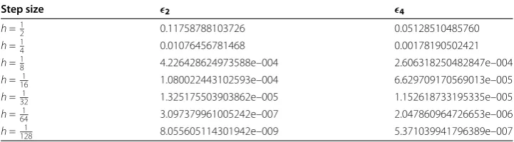
Example . Whena= –,a= .,b= ,b= .,ξ =  +t,τ = . In Table , the convergence of the exponential Euler method to Example . is described. Here we focus on the error at the endpointT= , , and the error is given asE|yn(ω) –x(T,ω)|, where

yn(ω) denotes the value of (.) at the endpoint. The expectation is estimated by averaging

random sample paths (ωi, ≤i≤,) over the interval [, ], that is,

e(h) =  ,

,

i=

_y_n(ωi) –x(T,ωi)

[image:16.595.117.478.632.732.2]

 .

Table 1 The global error of numerical solutions for the exponential Euler method

Step size 2 4

h=1

2 0.11758788103726 0.05128510485760

h=1

4 0.01076456781468 0.00178190502421

h=1₈ 4.226428624973588e–004 2.606318250482847e–004

h=₁₆1 1.080022443102593e–004 6.629709170569013e–005

h=₃₂1 1.325175503903862e–005 1.152618733195335e–005

h=₆₄1 3.097379961005242e–007 2.047860964726653e–006

(17)

[image:17.595.116.479.94.709.2]

(18)

In Table , we can see that the exponential Euler method to Example . is convergent, suggesting that (.) is valid.

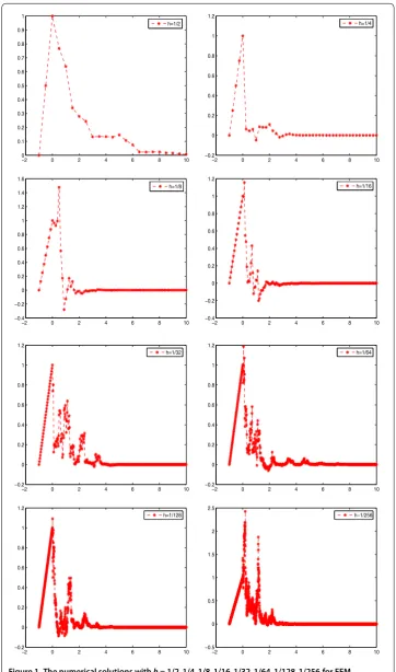
Example . Whena= –,a= ,b= ,b= .,ξ =  +t,τ = . We can show the stability of the exponential Euler method to (.). In Figure , all the curves decay toward to zero whenh= /,h= /,h= /,h= /,h= /,h= /,h= /,h= /. So we can consider that our experiments are consistent with our proved results in Section .

6 Conclusions

In this paper, we study convergence and exponential stability in mean square of the numer-ical solution for the exponential Euler method to semi-linear stochastic delay diﬀerential equations under the global Lipschitz condition and the linear growth condition. Firstly, Theorem . gives the exponential Euler approximation solution converging to the an-alytic solution with the strong order _ to SLSDDEs. Secondly, we give the exponential stability in mean square of the exact solution to SLSDDEs by using the deﬁnition of log-arithmic norm. Then we propose an explicit method to show that the exponential Euler method to SLSDDEs is proved to share the same stability for any step size. Finally, a nu-merical example is given to verify the method, the conclusion is correct. In Table , the convergence of the exponential Euler method to Example . is described. Here we focus on the error at the endpointT= , . In Figure , all the curves decay toward zero when h= /,h= /,h= /,h= /,h= /,h= /,h= /,h= /, and there is the same conclusion for any step size. So we can consider that our experiments are consistent with our proved results in Section .

Acknowledgements

I would like to thank the referees for their helpful comments and suggestions. The ﬁnancial support from the Youth Science Foundations of Heilongjiang Province of P.R. China (No.QC2016001) is gratefully acknowledged.

Competing interests

The author declares that no competing interests exist.

Authors’ contributions

All authors read and approved the ﬁnal manuscript.

Publisher’s Note

Springer Nature remains neutral with regard to jurisdictional claims in published maps and institutional aﬃliations.

Received: 7 April 2017 Accepted: 1 September 2017

References

1. Friedman, A: Stochastic Diﬀerential Equations and Applications, Vol. 1 and 2. Academic Press, New York (1975) 2. Higham, DJ, Mao, X, Yuan, C: Almost sure and moment exponential stability in the numerical simulation of stochastic

diﬀerential equations. SIAM J. Numer. Anal.41, 592-609 (2007)

3. Mao, X: Stochastic Diﬀerential Equations and Applications. Horwood, Chichester (1997)

4. Fuke, W, Xuerong, M: Convergence and stability of the semi-tamed Euler scheme for stochastic diﬀerential equations with non-Lipschitz continuous coeﬃcients. Appl. Math. Comput.228, 240-250 (2014)

5. Mao, X: The truncated Euler Maruyama method for stochastic diﬀerential equations. J. Comput. Appl. Math.290, 370-384 (2015)

6. Mao, X: Convergence rates of the truncated Euler Maruyama method for stochastic diﬀerential equations. J. Comput. Appl. Math.296, 362-375 (2016). doi:10.1016/j.cam.2015.09.035

7. Mao, X: Almost sure exponential stability in the numerical simulation of stochastic diﬀerential equations. SIAM J. Numer. Anal.53, 370-389 (2015)

8. Cao, WR, Liu, MZ, Fan, ZC: MS-stability of the Euler-Maruyama method for stochastic diﬀerential delay equations. Appl. Math. Comput.159, 127-135 (2004)

(19)

10. Mao, X: Numerical solutions of stochastic diﬀerential delay equations under the generalized Khasminskii-type conditions. Appl. Math. Comput.217, 5512-5524 (2011)

11. Wu*, K, Ding, X: Convergence and stability of Euler method for impulsive stochastic delay diﬀerential equations. Appl. Math. Comput.229, 151-158 (2014)

12. Mao, X: Exponential stability of equidistant Euler-Maruyama approximations of stochastic diﬀerential delay equations. J. Comput. Appl. Math.200, 297-316 (2007)

13. Kunze, M, Neerven, J: Approximating the coeﬃcients in semilinear stochastic partial diﬀerential equations. J. Evol. Equ.11, 577-604 (2011)