An efficient modification of the Hestenes Stiefel nonlinear conjugate gradient method with restart property

R E S E A R C H

Open Access

An efficient modification of the

Hestenes-Stiefel nonlinear conjugate

gradient method with restart property

Zabidin Salleh

_{and Ahmad Alhawarat}

*_{Correspondence:}

[email protected]

School of Informatics and Applied Mathematics, Universiti Malaysia Terengganu, Kuala Terengganu, Terengganu 21030, Malaysia

Abstract

The conjugate gradient (CG) method is one of the most popular methods to solve nonlinear unconstrained optimization problems. The Hestenes-Stiefel (HS) CG formula is considered one of the most efficient methods developed in this century. In addition, the HS coefficient is related to the conjugacy condition regardless of the line search method used. However, the HS parameter may not satisfy the global

convergence properties of the CG method with the Wolfe-Powell line search if the descent condition is not satisfied. In this paper, we use the original HS CG formula with a mild condition to construct a CG method with restart using the negative gradient. The convergence and descent properties with the strong Wolfe-Powell (SWP) and weak Wolfe-Powell (WWP) line searches are established. Using this condition, we guarantee that the HS formula is non-negative, its value is restricted, and the number of restarts is not too high. Numerical computations with the SWP line search and some standard optimization problems demonstrate the robustness and efficiency of the new version of the CG parameter in comparison with the latest and classical CG formulas. An example is used to describe the benefit of using different initial points to obtain different solutions for multimodal optimization functions.

Keywords: conjugate gradient method; Wolfe-Powell line search; Hestenes-Stiefel formula; restart condition; performance profile

1 Introduction

Consider the following form for the unconstrained optimization problem:

minf(x), x∈Rn, ()

wheref:Rn→Ris a smooth nonlinear function. To solve () using the conjugate gradient (CG) method, we normally use the following iterative method:

xk+=xk+αkdk, k= , , . . . , ()

where the starting pointx∈Rnis arbitrary andαk>  is the step length, which is

com-puted via a line search. The search directiondkis defined by

dk= –gk+βkdk–, k= , , . . . , ()

where gk=∇f(xk), βk is a scalar, and the steepest descent method is used as an initial

search direction,i.e.,

d= –g, k= . ()

The most well-known CG formulas are the following: Hestenes-Stiefel (HS) [],

β_kHS= g

T

k(gk–gk–) dT_k–(gk–gk–)

, ()

Fletcher-Reeves (FR) [],

β_kFR= gk



gk–

, ()

and Polak-Ribiere-Polyak (PRP) [],

β_kPRP=g

T

k(gk–gk–)

gk–

. ()

Theoretically, equations (), (), and () are similar if we use an exact line search,i.e.,

f(xk+αkdk) =minf(xk+αdk), α> , ()

and quadratic functions,i.e.,

f(x) =  x

T_Qx–bT_x,

whereQis a positive definite matrix andbis a vector. However, in numerical computa-tions and convergence analyses, the three main CG formulas are different if we use non-quadratic functions.

To obtain the step length, we have two types of line searches: exact line search as given by (), which is an expensive line search in terms of calculating the function and gradient evolutions, and inexact line search, which approximates the step length by reducing the function value and direction derivative. The inexact line search is inexpensive and inherits identical advantages as the exact line search. The most popular inexact line search is the Wolfe-Powell line search [, ], which is designed to approximate the suitable step length using the following equations:

f(xk+αkdk)≤f(xk) +δαkgkTdk ()

and

g(xk+αkdk)Tdk≥σgkTdk, ()

The strong version of the weak Powell (WWP) line search is the strong Wolfe-Powell (SWP) line search, which is given by () and

g(xk+αkdk)Tdk≤σgkTdk. ()

The difference between the WWP and SWP line searches is that the former no longer searches for the step length when the current iteration in () is far from the stationary point.

An important rule in the CG method is the descent property, which is given by

g_kTdk< . ()

If the CG formula inherits (), then the iterative formula in () absolutely reduces the function value in every iteration. It is clear from () thatf(xk+αkdk) –f(xk)≤δαkg_kTdk. If

the direction derivative (i.e.,gT

kdk) is negative, we obtain

f(xk+αkdk) =f(xk+) <f(xk).

Thus, () must be satisfied before using the Wolfe-Powell line search. If we extend () to the form

g_kTdk≤–cgk, k≥ andc> , ()

then () is called the sufficient descent condition.

The HS CG formula is related to the conjugacy condition regardless of the objective function and line search,i.e.,

d_kTgk–dkTgk–= . ()

If the CG formula inherits (), the efficiency will be better than other CG parameters that do not inherit this property. Dai and Liao [] proposed the following novel conjugacy condition for an inexact line search:

d_kTgk–dkTgk–= –tαk–gTkdk–, t> . ()

Using the criteria of an exact line search,g_kTdk–= , () reduces to the original conjugacy

condition ().

Because the PRP and HS formulas cannot satisfy the descent property when the SWP or WWP line searches are used, Gilbert and Nocedal [] use Powell’s [] suggestion to solve the convergence problem of the PRP method as follows:

β_kPRP+=max,β_kPRP,

β_kHS+=max,β_kHS.

Furthermore, [] makes the following suggestion:

βk=

⎧ ⎪ ⎨ ⎪ ⎩

–βFR

k , ifβkPRP< –βkFR, β_kPRP, if|β_kPRP| ≤β_kFR,

β_kFR, ifβ_kPRP>β_kFR.

Touati-Ahmed and Storey [] suggest the following hybrid method:

β_kTS= β

PRP

k , if ≤βkPRP≤βkFR, βFR

k , otherwise.

Several CG parameters that pertain to the PRP and HS formulas have been presented [– ]. Here, we denote the following CG formulas using the WYL family:

β_kWYL=g

T

k(gk–_gg_kk_–gk–)

gk–

, β_kNPRP=gk

_– gk gk–|gkgk–| gk–

,

β_kDPRP=gk

_– gk gk–|gkgk–| m|gT

kdk–|+gk–

, m≥.

The CG formulas in the WYL family are clearly positive and satisfy the global convergence with descent properties. However, this family does not inherit the restart property. Thus, the convergence rate is linear. For more about the convergence rate, we refer the reader to [].

Recently, Alhawaratet al.[] constructed the following CG formula with the restart property as follows:

β_kHPRP= β

PRP

k , ifgk>|gkTgk–|,

β_kNPRP, otherwise. ()

In addition, to learn about many versions of CG parameters related to classical CG meth-ods and their convergence properties, we refer the reader to [, ].

2 Motivation and the new modification

The Hestenes-Stiefel (HS) CG formula is considered one of the most efficient methods developed in this century. In addition, the HS coefficient is related to the conjugacy con-dition regardless of whether the line search used. However, the HS parameter may not satisfy the global convergence properties of the CG method with the Wolfe-Powell line search if the descent condition is not satisfied. Thus, in this section, we present the fol-lowing CG parameter:

β_kZA=

⎧ ⎨ ⎩

gk_–gT kgk–

dT_k–gk–dkT–gk–, ifgk

_>|gT kgk–|,

, otherwise.

()

The non-zero term of () can clearly be written as follows:

β_kZA≤ gk

_+|gT kgk–| d_kT_–gk–dkT–gk–

≤ gk d_kT_–gk–dTk–gk–

and

β_kZA> . ()

IfβZA

k = , the search direction becomes the steepest-descent method. In addition, ifgk=

, the stationary point is found. Thus, in the following analysis, we always suppose that

β_kZA>  andgk=  for allk≥.

To prove that the number of restarts in () is not too many by using different non-standard initial points, we compareβ_kZAwith the following modified PRP CG parameter:

β_kPRP∗=

g_kT(gk–gk–)

gk– , ifgk

_>|gT kgk–|,

, otherwise. ()

In the numerical results section, () restarted too many times by using non-standard dif-ferent initial points. In other words, the CG parameter in () uses the steepest-descent method several times to reach the optimum solution. However, by using the standard ini-tial points, PRP∗ becomes more efficient. Thus, in terms of the efficiency, () is not as efficient as () because the latter does not require as many times to restart.

The following algorithm describes the steps of using the CG method with () and SWP line search to obtain the solution for the optimization functions.

Algorithm 

Step . Initialization. Givenx, setk= .

Step . Ifgk ≤ε, then stop, where <ε. Step . Computeβkbased on ().

Step . Computedkbased on () and (). Step . Computeαkbased on () and (). Step . Update a new point based on ().

Step . Convergent test and stopping criteria: ifgk ≤ε, then stop; otherwise, go to Step  withk=k+ .

3 Global convergence properties for the

β

k method

Because we are interested in determining the stationary point for the nonlinear optimiza-tion funcoptimiza-tions that are bounded below and whose gradient is Lipschitz continuous, the following standard assumption is necessary.

Assumption 

I. The level set={x|f(x)≤f(x)}is bounded,i.e., there is a positive constantMsuch

that

x ≤M, ∀x∈.

II. In some neighborhoodNof,f is continuously differentiable, and its gradient is Lipschitz continuous,i.e., for allx,y∈N, there is a constantL> such that

This assumption implies that there is a positive constantBsuch that

g(u)≤B, ∀u∈N.

The following lemma is known as the Zoutendijk condition [], which is normally used to prove the convergence properties of CG formulas with the standard CG method. The global convergence indicates that a stationary point is obtained.

Lemma . Suppose that Assumptionholds.Consider the CG methods of forms()and

(),where the search direction satisfies the sufficient descent condition and the step length,

which is computed using the standard WWP line search.Then

∞

k=

(gT kdk) dk <∞.

The following two theorems demonstrate that () satisfies the descent condition with SWP and WWP line searches.

Theorem . Let the sequences{gk} and{dk}be generated by methods(), ()and()

with step lengthαk,which is computed using the SWP line searches()and()withσ<_; then the sufficient descent condition()holds for some c∈(, ).

Proof Multiplying () bygT

k, we have

g_kTdk=gkT(–gk+βkdk–) = –gk+βkgkTdk–. ()

Then we have the following two cases:

Case. IfgT

kdk–≤, then using (), we obtain

gT

kdk= –gk+βkZAgkTdk–< .

Case. IfgT_kdk–> , then divide both sides of () bygkand using (), we obtain

gT kdk

gk = – +β ZA

k gkTdk–.

Using () withσ< /, we obtain

gT kdk gk ≤– –

σgT k–dk–

(σ– )gT k–dk–

= – + σ ( –σ)< .

Letc=  – σ

(–σ), we obtain

g_kTdk≤–cgk.

The proof is complete.

Theorem . Assume the sequences{gk}and{dk}are generated using the methods(), ()

and()with step lengthαk,which is computed via the WWP line search given by()and

Proof IfgT

kdk–≤, then the proof is similar to Case  in Theorem .. IfgkTdk–> , from

(), we have

g_kTdk =gkT(–gk+βkdk–) = –gk+βkgTkdk–

≤–gk+ gk



dT

k–gk–dTk–gk–

g_kTdk–

= 

d_kT_–gk–dTk–gk–

–gkdT_k–gk+gkdTk–gk–+ gkgkTdk–

= 

dT

k–(gk–gk–)

gkd_kT_–gk–+gkgkTdk–

= 

dT

k–(gk–gk–)

gkd_kT_–gk–+gkdkT–gk––gkdTk–gk–+gkgkTdk–

= 

d_kT_–(gk–gk–)

gkd_kT_–(gk–gk–) + gkdkT–gk–

≤ gk+gk

_dT k–gk–

(σ– )dT_k–gk–

≤ gk+gk



(σ– ).

Dividing both sides bygk, we obtain

gT kdk gk ≤ +

 (σ– ).

Letc= – +_(–_σ); then we obtain

g_kTdk≤–cgk.

The proof is complete.

Gilbert and Nocedal [] presented a useful property to prove the global convergence properties for the methods that pertain to the PRP (HS) formula. The property is as fol-lows.

Property∗ Consider a method of the form given by () and () and suppose that

 <γ ≤ gk ≤ ¯γ. ()

We say that the method has Property∗if there are constantsb>  andλ>  such that for allk≥, we obtain|βk| ≤b; ifxk–xk– ≤λ, then

|βk| ≤ 

b.

Lemma . Consider the CG method as defined in(), (),and()and the step length computed using the WWP line search.If the equation in()and Assumptionhold,then β_kZAsatisfies Property∗.

Proof Assume thatb=_(–_σγ¯₎_cγ andλ=

(–σ)cγ

Lγ¯b . Thenb>  andλ> . Using () and

The-orem ., we obtain

d_kT_–(gk–gk–)≥(σ– )gkT–dk–≥c( –σ)gk–.

Using () and Assumption , we obtain

β_kZA= g

T

k(gk–gk–)

dT

k–(gk–gk–)

≤gk+|gkTgk–|

c( –σ)gk– ≤

γ¯

c( –σ)γ =b.

Ifxk–xk– ≤λ, then

β_kZA=gk

_–gT kgk– dT_k–(gk–gk–)

≤gkgk–gk–

c( –σ)gk– ≤

Lλγ¯ c( –σ)γ =

 b.

The proof is complete.

The proof of the forthcoming lemmas and Theorem . originally can be found in []. However, we present it here for readability. The following lemma shows that if the CG formula satisfies Property∗, then the fraction of steps cannot be too small.

Lemma . Assume that Assumptionholds.Assume that the sequences{gk}and{dk}are generated by Algorithm,whereαkis computed using the WWP line search,in which the sufficient descent condition()holds,and assume that the method has Property∗.Suppose alsogk ≥γfor someλ> .Then there existsλ> such that for any∈Nand any index k,there is an index k>kthat satisfies

κ_kλ_,>λ ,

whereκ_kλ_,={i∈N:k≤i≤k+– ,si>λ},Ndenotes the set of positive integers,and |κλ

k,|denotes the number of elements inκkλ,.

Lemma . Suppose that Assumptionholds.Assume that the sequences{gk}and{dk} are generated by Algorithm,whereαkis computed using the WWP line search,and that the sufficient descent condition()holds.Ifβk≥and()holds,then dk= and

∞

k=

uk+–uk<∞, where uk= dk dk.

Proof Based on Lemma ., we prove the theorem by contradiction. Defineui:=d_di_i. For

any two indicesl,kwithl≥k, we have

xl–xk–=

l

i=k

si–ui–=

l

i=k

si–uk–+

l

i=k

si–(ui––uk–),

wheresi–=xi–xi–.

Taking the norms,

l

i=k

si– ≤ xl+xk–+

l

i=k

si–ui––uk–.

Using Assumption , we know that sequence{xk}is bounded, and there is a positive con-stantηsuch thatxk ≤ηfor allk≥. Thus,

xl+xk– ≤η,

which implies that

l

i=k

si– ≤η+

l

i=k

si–ui––uk–. ()

Assume thatλ>  is given by Lemma .. Following the notation of this lemma, we define

:= η λ .

From Lemma ., we can find an indexksuch that

∞

k≥k

ui–ui–<



. ()

With thisandk, Lemma . gives an indexk≥ksuch that

κ_kλ_,>

. ()

Next, according to the Cauchy-Schwarz inequality and (), we see that for any index

i∈[k,k+– ],

ui––uk– ≤

i–

j=k

uj–uj–

≤(i–k)/

_i–

j=k

uj–uj–

By this relation, () and (), withl=k+– , we have

η≥



k+–

i=k

si–>

λ

κ λ

k,>

λ

 .

Thus,< η/λ, which contradicts the definition of. The proof is complete.

Using Lemmas ., ., and . and Theorem ., the global convergence of Algorithm  with the Wolfe-Powell line search is similarly established to that in Theorem . in []. Therefore, the proof of the following theorem is omitted, and we present the following theorems without proof.

Theorem . Suppose that Assumptionholds.Consider the CG method of forms(), ()

and(),whereαkis computed using the WWP line search;thenlimk→∞infgk= .

Theorem . Suppose that Assumptionholds.Consider the CG method of forms(), () and (), where αk is computed using the SWP line search with  <σ < /; then lim_k→∞infgk= .

4 Numerical results and discussion

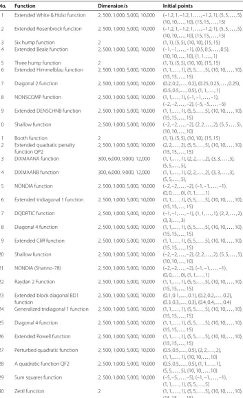
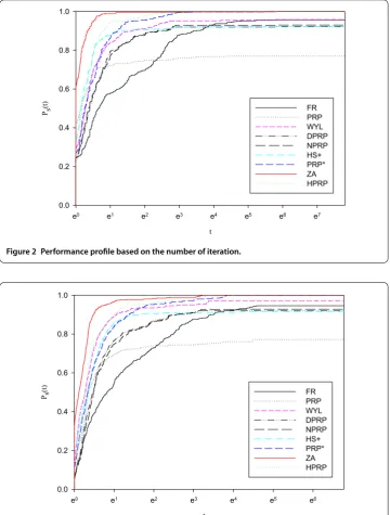
To test the efficiency and robustness of the new method (), some standard test functions were selected from CUTE [] and Andrei [], as summarized in Table . We performed a comparison with other CG methods, which included the WYL family, PRP∗, HPRP, PRP, HS+, FR, and ZA parameters. The stopping criterion wasgk ≤–_{for all algorithms.}

The initial pointx∈Rnis arbitrary. As shown in Table , we used different initial points

based on the original standard points. We notice from the numerical results that differ-ent initial points almost had differdiffer-ent stationary points for the multimodal functions. In addition, the efficiency of the algorithm depended on the initial points for every function. For example, the efficiency of the FR algorithm with the extended Rosenbrock function and the initial point (–., , –., , . . . , –., ) is different from that with (, , . . . , ) or (, , . . . , ) as the initial point. Moreover, the initial point determines the value of the CG formula based on Powell []; for example, the PRP or HS parameter fails to obtain the solution if its value is negative. In contrast, if we use another initial point, the value of PRP is non-negative and satisfies the descent property. This result motivated us to further study the initial points. Moreover, different dimensions were used for every function, and the dimension range was [, ,].

We present Himmelblau’s function (Figure ), which is a multimodal function to test the efficiency of the optimization algorithms. The function is defined as follows:

f(x,y) =x+y– +x+y– .

Table 1 A list of test problem functions

No. Function Dimension/s Initial points

1 Extended White & Holst function 2, 500, 1,000, 5,000, 10,000 (–1.2, 1, –1.2, 1,. . ., –1.2, 1), (5, 5,. . ., 5),

(10, 10,. . ., 10), (15, 15,. . ., 15)

2 Extended Rosenbrock function 2, 500, 1,000, 5,000, 10,000 (–1.2, 1, –1.2, 1,. . ., –1.2, 1), (5, 5,. . ., 5),

(10, 10,. . ., 10), (15, 15,. . ., 15)

3 Six hump function 2 (1, 1), (5, 5), (10, 10), (15, 15)

4 Extended Beale function 2, 500, 1,000, 5,000, 10,000 (–1, –1,. . ., –1), (0.5, 0.5,. . ., 0.5),

(10, 10,. . ., 10), (1, 1,. . ., 1)

5 Three hump function 2 (1, 1), (5, 5), (10, 10), (15, 15)

6 Extended Himmelblau function 2, 500, 1,000, 5,000, 10,000 (1, 1,. . ., 1), (5, 5,. . ., 5), (10, 10,. . ., 10),

(15, 15,. . ., 15)

7 Diagonal 2 function 2, 500, 1,000, 5,000, 10,000 (0.2, 0.2,. . ., 0.2), (0.25, 0.25,. . ., 0.25),

(0.5, 0.5,. . ., 0.5), (1, 1,. . ., 1)

8 NONSCOMP function 2, 500, 1,000, 5,000, 10,000 (1, 1,. . ., 1), (–1, –1,. . ., –1),

(–2, –2,. . ., –2), (–5, –5,. . ., –5)

9 Extended DENSCHNB function 2, 500, 1,000, 5,000, 10,000 (1, 1,. . ., 1), (5, 5,. . ., 5), (10, 10,. . ., 10),

(15, 15,. . ., 15)

10 Shallow function 2, 500, 1,000, 5,000, 10,000 (–2, –2,. . ., –2), (2, 2,. . ., 2), (5, 5. . ., 5),

(10, 10,. . ., 10)

11 Booth function 2 (1, 1), (5, 5), (10, 10), (15, 15)

12 Extended quadratic penalty

function QP2

2, 500, 1,000, 5,000, 10,000 (2, 2,. . ., 2), (5, 5,. . ., 5), (10, 10,. . ., 10),

(15, 15,. . ., 15)

13 DIXMAANA function 300, 6,000, 9,000, 12,000 (1, 1,. . ., 1), (2, 2,. . ., 2), (3, 3,. . ., 3),

(5, 5,. . ., 5),

14 DIXMAANB function 300, 6,000, 9,000, 12,000 (1, 1,. . ., 1), (2, 2,. . ., 2), (3, 3,. . ., 3),

(5, 5,. . ., 5),

15 NONDIA function 2, 500, 1,000, 5,000, 10,000 (–2, –2,. . ., –2), (–1, –1,. . ., –1),

(0, 0,. . ., 0), (1, 1,. . ., 1)

16 Extended tridiagonal 1 function 2, 500, 1,000, 5,000, 10,000 (1, 1,. . ., 1), (5, 5,. . ., 5), (10, 10,. . ., 10),

(15, 15,. . ., 15)

17 DQDRTIC function 2, 500, 1,000, 5,000, 10,000 (–1, –1,. . ., –1), (1, 1,. . ., 1), (2, 2,. . ., 2),

(3, 3,. . ., 3)

18 Diagonal 4 function 2, 500, 1,000, 5,000, 10,000 (1, 1,. . ., 1), (5, 5,. . ., 5), (10, 10,. . ., 10),

(15, 15,. . ., 15)

19 Extended Cliff function 2, 500, 1,000, 5,000, 10,000 (1, 1,. . ., 1), (5, 5,. . ., 5), (10, 10,. . ., 10),

(15, 15,. . ., 15)

20 Shallow function 2, 500, 1,000, 5,000, 10,000 (–2, –2,. . ., –2), (2, 2,. . ., 2), (5, 5,. . ., 5),

(10, 10,. . ., 10)

21 NONDIA (Shanno-78) 2, 500, 1,000, 5,000, 10,000 (–2, –2,. . ., –2), (–1, –1,. . ., –1),

(0, 0,. . ., 0), (1, 1,. . ., 1)

22 Raydan 2 Function 2, 500, 1,000, 5,000, 10,000 (1, 1,. . ., 1), (5, 5,. . ., 5), (10, 10,. . ., 10),

(15, 15,. . ., 15)

23 Extended block diagonal BD1

function

2, 500, 1,000, 5,000, 10,000 (0.1, 0.1,. . ., 0.1), (0.2, 0.2,. . ., 0.2),

(0.3, 0.3,. . ., 0.3), (0.4, 0.4,. . ., 0.4)

24 Generalized tridiagonal 1 function 2, 500, 1,000, 5,000, 10,000 (1, 1,. . ., 1), (5, 5,. . ., 5), (10, 10,. . ., 10),

(15, 15,. . ., 15)

25 Diagonal 4 function 2, 500, 1,000, 5,000, 10,000 (1, 1,. . ., 1), (5, 5,. . ., 5), (10, 10,. . ., 10),

(15, 15,. . ., 15)

26 Extended Powell function 2, 500, 1,000, 5,000, 10,000 (1, 1,. . ., 1), (5, 5,. . ., 5), (10, 10,. . ., 10),

(15, 15,. . ., 15)

27 Perturbed quadratic function 2, 500, 1,000, 5,000, 10,000 (0.5, 0.5,. . ., 0.5), (2, 2,. . ., 2),

(1, 1,. . ., 1), (10, 10,. . ., 10)

28 A quadratic function QF2 2, 500, 1,000, 5,000, 10,000 (0.5, 0.5,. . ., 0.5), (1, 1,. . ., 1),

(5, 5,. . ., 5), (10, 10,. . ., 10)

29 Sum squares function 2, 500, 1,000, 5,000, 10,000 (–5, –5,. . ., –5), (–1, –1,. . ., –1),

(1, 1,. . ., 1), (5, 5,. . ., 5)

30 Zettl function 2 (1, 1,. . ., 1), (5, 5,. . ., 5), (10, 10,. . ., 10),

Figure 1 Himmelblau’s function.

Table 2 The initial points corresponding the optimal points with the Himmelblau function

Initial point The optimal solution The function value

(1, 1) (3, 2) f(3, 2) = 0

(–1, –1) (3.5844, –1.8481) f(3.5844, –1.8481) = 0

(10, 10) (–3.7793, –3.2832) f(–3.7793, –3.2832) = 0

(–5, –5) (–2.8051, 3.1313) f(–2.8051, 3.1313) = 0

The performance results are shown in Figures  and  with a performance profile intro-duced by Dolan and Moré [].

This performance measure was introduced to compare a set of solvers S on a set of problemsF. Assuming that there arenssolvers andnf problems inSandF, respectively.

Then the measuretf,sis defined as the required number of iterations or CPU time to solve

problemf using solvers. To create a baseline for comparison, the performance of solver

son problemf is scaled by the best performance of any solver inSon the problem using the ratio

rf,s=

tf,s min{tf,s:s∈S}

.

Suppose that a parameterrM≥rf,sfor allf,sis selected.rf,s=rM if and only if solvers

does not solve problemf.

Because we would like to obtain an overall assessment of the performance of a solver, we defined the measure

Ps(t) =



nf

Figure 2 Performance profile based on the number of iteration.

Figure 3 Performance profile based on the CPU time.

Thus,Ps(t) is the probability for solvers∈Sthat the performance ratiorf,sis within a factor t∈Rof the best possible ratio. If we define functionpsas the cumulative distribution

function for the performance ratio, then the performance measure fs:R→[, ] for a

solver is non-decreasing and piecewise continuous from the right. The value offs() is the

probability that the solver has the best performance of all solvers. In general, a solver with high values off(t), which appears in the upper right corner of the figure, is preferable.

Although the PRP and HS methods are efficient, both of them have theoretical problems; thus, the number of solved function using the PRP formula does not exceed %. The HS+ formula also has theoretical problem when the direction derivative is positive; hence, it may not satisfy the descent property with the SWP line search. Thus, the percentage value of solved functions using the HS+ formula is approximately %. The FR formula satisfies the descent property and convergence property, but we terminated the program several times because it is cyclic without reaching the solution. For all algorithms, the time limit to obtain the solution was  seconds.

5 Conclusion

In this paper, we used the HS CG formula with the restart. The global convergence and descent properties were established with WWP and SWP line searches. The numerical results demonstrate that the new modification is better than other CG parameters.

Competing interests

The authors declare that they have no competing interests.

Authors’ contributions

All authors contributed equally to the writing of this paper. All authors read and approved the final version of this paper.

Acknowledgements

The authors are grateful to the editor and the anonymous reviewers for their valuable comments and suggestions, which have substantially improved this paper. In addition, we acknowledge the Ministry of Higher Education Malaysia and Universiti Malaysia Terengganu; this study was partially supported under the Fundamental Research Grant Scheme (FRGS) Vote no. 59347.

Received: 8 November 2015 Accepted: 18 March 2016

References

1. Hestenes, MR, Stiefel, E: Methods of conjugate gradients for solving linear systems. J. Res. Natl. Bur. Stand.49(6),

409-436 (1952)

2. Fletcher, R, Reeves, CM: Function minimization by conjugate gradients. Comput. J.7(2), 149-154 (1964)

3. Polak, E, Ribiere, G: Note sur la convergence de méthodes de directions conjuguées. ESAIM: Math. Model. Numer.

Anal.3(R1), 35-43 (1969)

4. Wolfe, P: Convergence conditions for ascent methods. SIAM Rev.11, 226-235 (1968)

5. Wolfe, P: Convergence conditions for ascent methods. II: some corrections. SIAM Rev.13, 185-188 (1971)

6. Dai, Y-H, Liao, L-Z: New conjugacy conditions and related nonlinear conjugate gradient methods. Appl. Math. Optim.

43(1), 87-101 (2001)

7. Gilbert, JC, Nocedal, J: Global convergence properties of conjugate gradient methods for optimization. SIAM J.

Optim.2(1), 21-42 (1992)

8. Zoutendijk, G: Nonlinear programming, computational methods. Integer Nonlinear Program.143(1), 37-86 (1970)

9. Moré, JJ, Thuente, DJ: On line search algorithms with guaranteed sufficient decrease. Mathematics and Computer Science Division Preprint MCS-P153-0590, Argonne National Laboratory, Argonne, IL (1990)

10. Touati-Ahmed, D, Storey, C: Efficient hybrid conjugate gradient techniques. J. Optim. Theory Appl.64, 379-397 (1990)

11. Wei, Z, Yao, S, Liu, L: The convergence properties of some new conjugate gradient methods. Appl. Math. Comput.

183(2), 1341-1350 (2006)

12. Zhang, L: An improved Wei-Yao-Liu nonlinear conjugate gradient method for optimization computation. Appl. Math.

Comput.215(6), 2269-2274 (2009)

13. Dai, Z, Wen, F: Another improved Wei-Yao-Liu nonlinear conjugate gradient method with sufficient descent property.

Appl. Math. Comput.218(14), 7421-7430 (2012)

14. Sun, W, Yuan, YX: Optimization Theory and Methods: Nonlinear Programming, vol. 1. Springer, Berlin (2006) 15. Alhawarat, A, Mamat, M, Rivaie, M, Salleh, Z: An efficient hybrid conjugate gradient method with the strong

Wolfe-Powell line search. Math. Probl. Eng.2015, Article ID 103517 (2015)

16. Yuan, G, Meng, Z, Li, Y: A modified Hestenes and Stiefel conjugate gradient algorithm for large-scale nonsmooth

minimizations and nonlinear equations. J. Optim. Theory Appl.168(1), 129-152 (2016)

17. Alhawarat, A, Mamat, M, Rivaie, M, Mohd, I: A new modification of nonlinear conjugate gradient coefficients with

global convergence properties. Int. J. Math. Comput. Stat. Nat. Phys. Eng.8(1), 54-60 (2014)

18. Bongartz, I, Conn, AR, Gould, N, Toint, PL: CUTE: constrained and unconstrained testing environment. ACM Trans.

Math. Softw.21(1), 123-160 (1995)

19. Andrei, N: An unconstrained optimization test functions collection. Adv. Model. Optim.10(1), 147-161 (2008)

20. Powell, MJD: Nonconvex Minimization Calculations and the Conjugate Gradient Method. Springer, Berlin (1984)

21. Dolan, ED, Moré, JJ: Benchmarking optimization software with performance profiles. Math. Program.91(2), 201-213