Time adaptive dynamic software reconfiguration for embedded software

(1)

Time-Adaptive Dynamic Software Reconfiguration for

Embedded Software

Serena Fritsch

A Thesis submitted to the University of Dublin, Trinity College in fulfillment of the requirements for the degree of

Doctor of Philosophy (Computer Science)

(2)

Declaration

I, the undersigned, declare that this work has not previously been submitted to this or any other University, and that unless otherwise stated, it is entirely my own work.

Serena Fritsch

(3)

Permission to Lend and/or Copy

I, the undersigned, agree that Trinity College Library may lend or copy this Thesis upon request.

Serena Fritsch

(4)

Acknowledgements

It was the best of times, it was the worst of times, it was the age of wisdom, it was the age of foolishness

Charles Dickens

First and foremost, I thank my supervisor Dr. Siobh´an Clarke for her guidance, and support over the years. I very much appreciate her motivation, feedback, and endless patience during my Ph.D. studies.

I also thank the other members of Lero in the Distributed Systems Group for the good collaboration, and the fruitful discussions, which helped to shape my research.

I express my gratitude to all those who read and reviewed my thesis and provided valuable suggestions, especially Ivana Dusparic, Jenny Munnelly, Melanie Bouroche, Raymond Cunningham, Andronikos Nedos, Ashley Sterritt, and Brendan Cody-Kenny. A big thank you also to Gregor Schiele for feedback on earlier stages of this research.

To all past and present members in the Distributed Systems Group, thank you for making it such a great and lively research environment to be in. A big thank you goes especially to my room mates of Lloyd 008 for lively discussions (not only) about work, and for being great collegues. I also thank the Science Foundation Ireland, for sponsoring my research.

(5)

fellows: As’ad Salkham, Ashley Sterritt, Bartek Biskupski, Farrukh Mirza, Guoxiang Yang, Ivana Dusparic, Marcin Karpinski, Melanie Bouroche, Mithileash Mohan, and Warren Kenny. A big thank you also to Aline Senart, Ibrahim Tawfik, Liliana Abudalo, Ilona Biskupska, Malgorzata Jaksik, Maribel Salvador, Michael Moltenbrey, Peter Otte, Sabine Horn, and Steffen Maier, for their friendship and contact to the outside world. There are many more names to be mentioned here, but i hope you all know who you are.

And finally, thank you to my family for their continuous love, support, and encour-agement.

Serena Fritsch

(6)

(7)

Summary

Reactive embedded systems, such as sensor nodes, or real-time control systems, are em-bedded into and interact with a physical environment for controlling and measuring pur-poses. When deployed in environments with changing requirements and unpredictable events, these systems need to adapt their software to maintain a desired level of func-tionality. As these systems are generally long lived, they need to provide means for allowing software adaptations such as introducing new, or improving old functionality. There are many static software adaptation techniques, but high reliability and durability constraints for reactive embedded systems make stopping and changing their structure or behaviour offline undesirable. Dynamic software reconfiguration is needed to allow such changes to happen while the system, or parts of the system, remain functional.

(8)

Transactional reconfiguration approaches complete the reconfiguration without con-sideration of the incoming events and their processing deadline. However, this might lead to a missed event deadline with implications for the system’s overall timeliness. Preemptive reconfiguration approaches stop any reconfiguration activity and directly process an incoming event, which results in a timely computation of the event. However, this might delay a reconfiguration indefinitely if many incoming events occur consecu-tively. A reconfiguration model targeting reactive, embedded systems should fulfill two requirements: The model should meet the processing deadline of incoming events, while at the same time it should make progress towards a completion of the reconfiguration. The research question that emerges is what techniques are neccessary to realise such a reconfiguration model.

To address this question, this thesis introduces TimeAdapt, a time-adaptive recon-figuration model. Input to the model is the current software conrecon-figuration, an event’s processing deadline, and the remaining reconfiguration activities. Based on that input, the model determines how much of the reconfiguration can still be executed to reach a safe configuration within the given processing deadline. The core of the model is a parti-tioning of a reconfiguration process sequence into sub-sequences of reconfiguration tasks that are safe to be interrupted and sub-sequences that must be executed atomically to reach a valid safe intermediate system configuration. The reconfiguration model is de-fined for embedded software that follows the data-flow based computational model. This model was chosen as it is a well-defined mathematical model for concurrent computations and is general enough to describe distributed and local software architectures.

(9)

architec-ture.

(10)

Publications Related to this Ph.D.

[1] Shane Brennan, Serena Fritsch, Yu Liu, Ashley Sterritt, Jorge Fox, Eamon Line-han, Cormac Driver, Rene Meier, Vinny Cahill, William Harrison, Siobh´an Clarke, “A Framework for Flexible and Dependable Service-Oriented Embedded Systems”, to appear in the 7th Book on Architecting Dependable Systems (ADS 7), Springer, 2010

[2] Serena Fritsch, and Siobh´an Clarke, “TimeAdapt: Timely Execution of Dynamic Software Reconfigurations”. Proceedings of the 5th Middleware Doctoral Sympo-sium (Middleware 2008), pages 13-18, December 2008, Leuven, Belgium.

[3] Serena Fritsch, Aline Senart, Douglas C. Schmidt, and Siobh´an Clarke. “Time-Bounded Dynamic Adaptation for Automotive System Software”. Proceedings of the 30th International Conference on Software Engineering (ICSE), Experience Track on Automotive Systems, May 2008, Leipzig, Germany.

(11)

List of Tables

2.1 Properties of execution models . . . 20

2.2 Features of Runes reconfiguration model . . . 28

2.3 Features of Think reconfiguration model . . . 30

2.4 Features of DynamicCon reconfiguration model . . . 32

2.5 Features of DynaQoS-RDF reconfiguration model . . . 35

2.6 Features of Djinn reconfiguration model . . . 38

2.7 Features of PBO reconfiguration model . . . 40

2.8 Features of Molecule reconfiguration model . . . 42

2.9 Features of NecoMan reconfiguration model . . . 44

2.10 Comparison of system model properties . . . 46

2.11 Comparison of reconfiguration model properties . . . 47

2.12 Comparison of execution model features . . . 48

2.13 Comparison of constraint properties . . . 50

2.14 Comparison summary . . . 51

3.1 Overview of pessimistic mode parameters . . . 85

3.2 Overview of optimistic mode parameters . . . 93

3.3 Requirements vs. TimeAdapt features . . . 102

5.1 Summary of TimeAdapt evaluation experiments . . . 132

(16)

5.3 Percentage of deadlines met . . . 135

5.4 Mapping between figures and experiment settings . . . 135

5.5 Percentage of reconfiguration actions remaining . . . 141

5.6 Mapping between figures and experiment settings . . . 142

5.7 Experiment 2: Parameter Setting . . . 150

5.10 Deadline values associated with events . . . 167

C.1 Statistical values for low event arrival time . . . 196

C.2 Statistical values for medium event arrival time . . . 196

C.3 Statistical values for high event arrival time . . . 196

C.4 Statistical values for low event arrival rate . . . 197

C.5 Statistical values for medium event arrival rate . . . 198

(17)

List of Figures

1.1 Execution of reconfiguration actions depending on event processing

dead-line td . . . 9

2.1 Timing analysis of reconfiguration process (Rasche & Polze, 2003) . . . . 18

2.2 The non-blocking reconfiguration approach (Schneider, 2004) . . . 32

2.3 Reconfiguration of a single mobile unit to different communication mech-anisms (Mitchell et al., 1998) . . . 36

2.4 Communication between PBOs (Issel, 2006) . . . 38

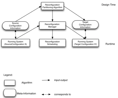
3.1 TimeAdapt Design . . . 56

3.2 Original actor configuration and the executed reconfiguration sequence . . 68

3.3 Unsafe software configuration . . . 69

3.4 Safe software configuration . . . 69

3.5 TimeAdapt reconfiguration model overview . . . 73

3.6 Reconfiguration partitioning inputs and outputs . . . 74

3.7 Partitioning algorithm . . . 76

3.8 Partitioning example: Interface-changing actions . . . 79

3.9 Partitioning example: Non-interface changing and interface-changing ac-tions . . . 80

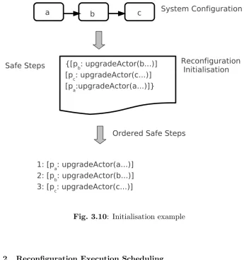
3.10 Initialisation example . . . 82

(18)

3.12 System configuration before optimistic scheduling mode executes . . . 88

3.13 System configuration after execution of a single reconfiguration action . . 89

3.14 Reconfiguration action phases . . . 90

3.15 Different outcomes for the optimistic scheduling mode . . . 94

3.16 Timing behaviour of TimeAdapt . . . 97

3.17 Point in time of incoming events . . . 98

4.1 TimeAct System Architecture . . . 104

4.2 TimeAct Component Model . . . 106

4.3 TimeAct Component Model: User-defined classes . . . 111

4.4 TimeAdapt Reconfiguration model implementation . . . 113

4.5 Reconfiguration sequence generation . . . 119

4.6 Non-interrupted reconfiguration execution . . . 121

4.7 Interrupted reconfiguration execution . . . 123

5.1 Temperature sensor scenario realised on embedded platform . . . 128

5.2 Percentage of deadlines met for low event arrival rate and deadlines range from 0.15 ms to 100 ms . . . 136

5.3 Percentage of deadlines met for medium event arrival rate and deadlines range from 0.15 ms to 100 ms . . . 137

5.4 Percentage of deadlines met for high event arrival rate and deadlines range from 0.15 ms to 100 ms . . . 138

5.5 Percentage of deadlines met for medium event arrival rate and deadlines range from 0.15 ms to 20 ms . . . 139

5.6 Percentage of deadlines met for a very high event arrival rate and deadlines range from 0.15 ms to 20 ms . . . 140

5.7 Percentage of remaining actions for low event arrival rate . . . 143

5.8 Percentage of remaining actions for medium event arrival rate . . . 144

(19)

5.10 Pessimistic mode: Number of remaining actions for medium event arrival rate and two consecutive events . . . 146 5.11 Optimistic mode: Number of remaining actions for medium event arrival

rate and two consecutive events . . . 147 5.12 Pessimistic Mode: Number of remaining actions for very high event arrival

rate and two consecutive events . . . 148 5.13 Optimistic Mode: Number of remaining actions for very high event arrival

rate and two consecutive events . . . 149 5.14 Pessimistic Mode: Percentage of deadlines met for low event arrival rate . 152 5.15 Optimistic Mode: Percentage of deadlines met for low event arrival rate . 153 5.16 Pessimistic Mode: Percentage of remaining actions for low event arrival

rate . . . 154 5.17 Optimistic Mode: Percentage of remaining actions for low event arrival

rate . . . 155 5.18 Percentage of deadlines met for low event arrival rate . . . 159 5.19 Percentage of remaining actions for low event arrival rate . . . 160 5.20 Pessimistic Mode: Percentage of deadlines met for medium event arrival

rate and homogeneous deadlines . . . 163 5.21 Optimistic Mode: Percentage of deadlines met for medium event arrival

rate and homogeneous deadlines . . . 164 5.22 Pessimistic Mode: Percentage of remaining actions for medium event

ar-rival rate and homogeneous deadlines . . . 165 5.23 Optimistic Mode: Percentage of remaining actions for medium event

ar-rival rate and homogeneous deadlines . . . 166 5.24 Pessimistic Mode: Percentage of deadlines met for medium event arrival

rate and heterogeneous deadlines . . . 167 5.25 Optimistic Mode: Percentage of deadlines met for medium event arrival

(20)

5.26 Pessimistic Mode: Percentage of remaining actions for medium event ar-rival rate and heterogeneous deadlines . . . 169 5.27 Optimistic Mode: Percentage of remaining actions for medium event

(21)

Chapter 1

Introduction

(22)

aims to meet the processing deadline of incoming events, while at the same time, making progress towards completion of a reconfiguration. This introductory chapter provides the background and motivation for this work, introduces the proposed approach to the dynamic reconfiguration of embedded software, presents the contributions of this thesis and outlines the remainder of this thesis.

1.1 Background

Embedded systems, such as sensors in a sensor network or real-time control systems, are reactive (Rutten, 2008). Unlike transformational or interactive systems, reactive systems are computer systems that continuously react to their environment at a speed determined by the environment (Halbwachs, 1993). In contrast to general-purpose soft-ware, embedded software interacts with the physical world rather than dealing with the transformation of data (Lee, 2002). According to Lee (2002), the software of reactive embedded systems has some distinctive features such as:

• Concurrency: A typical embedded application consists of several parallel

activ-ities that interact with each other and with the external environment (Cheong & Liu, 2005). Each of these activities must react to stimuli from a variety of sensors.

• Event-driven Computations: The software is event-driven, i.e., conceptually

concurrent components are activated by incoming events.

• Timeliness of Computations: Many of these systems control critical entities

and incoming events, and actuators, must be executed within a time bound.

• Liveness Property: In embedded systems, liveness is a critical issue as programs

must not terminate or block waiting for events that may never occur (Lee, 2002). Termination is considered a failure and should be avoided.

(23)

their relationships and properties that allows an embedded system to operate correctly according to its architecture” (Perrson, 2009). Traditionally, this configuration was statically determined at system design-time and did not change during system runtime. However, the trend towards open embedded systems requires the dynamic change of con-figurations (Baresi et al., 2006). These systems are exposed to changing environments and to changes that were not envisioned at design time. The liveness requirements of reactive embedded systems makes stopping the system and changing its software config-uration offline undesirable (Lee, 2002). Consequently, dynamic software reconfigconfig-uration is needed to allow such changes to occur while the software remains functional.

(24)

component-based embedded application software that runs on top of a single-processor embedded system (Cheong, 2007). Examples for this kind of software are sensing ap-plications on a single sensor node. For the rest of this thesis, this kind of software is referred to as embedded software. However, the approach can also be generalised to lower-level system software, such as operating system software (Friedrich et al., 2001), or middleware software (Schmidt, 2002).

1.2 Motivation

Dynamic reconfiguration in embedded software occurs while the underlying system re-acts to incoming events such as physical events, user commands, and messages from other systems (Cheong et al., 2003). For example, while the reconfiguration is executed, the underlying hardware raises an interrupt. However, these incoming events have the potential to cause conflict between two requirements. Firstly, as many of these systems operate in real-time, event processing needs to be started within the so-called processing deadline (Lee, 2002). Secondly, a reconfiguration may be required to react to current prevailing conditions and therefore it should complete as soon as possible to maintain acceptable quality of service.

Current reconfiguration models for embedded software can be classified according to their execution model into transactional or preemptive approaches, depending on how they address the two conflicting requirements of a reconfiguration.

(25)

reconfigurations within static time bounds that are either dictated by the characteris-tics of the underlying hardware or defined by the application developer. However, all these approaches do not react to previously unknown incoming events. As a result, the processing deadlines of these events might be missed with implications for the system’s overall timeliness.

In contrast to transactional approaches, preemptive reconfiguration approaches allow the interruption of an ongoing reconfiguration (Zhao & Li, 2007b). These approaches can directly react to an event by preempting the ongoing reconfiguration and processing the event. A precondition for these approaches is that the reconfiguration can be directly pre-empted. These approaches do not support the reconfiguration of stateful software entities, as this implies reconfiguration actions that are not instantaneous. However, in the presence of many incoming events, the completion of a reconfiguration is potentially delayed indefinitely. As a result, these approaches do not meet the requirement for a timely completion of the reconfiguration process.

1.2.1 Challenges for Dynamic Software Reconfiguration in Embedded

Software

Embedded software imposes additional challenges for reconfiguration models with re-spect to the following factors that need to be considered: Reaching quiescent state, maintaining structural dependency relationships, and scheduling reconfigurations.

• Reaching quiescent stateA pre-condition for dynamic software reconfiguration

(26)

Embedded software, which consists of multiple threads of execution, extends the time it takes until a quiescent state is reached. It also affects the type of approach suitable for reaching a quiescent state. For example, using an approach that reaches a quiescent state by observing system execution is not feasible as execution threads never terminate and block reconfiguration start (Wegdam, 2003).

• Maintaining structural dependency relationshipsDependency relationships

between software entities constrain the structure of the software (Almeida et al., 2001). Dynamic software reconfiguration must not break the dependencies between collaborating software entities, as otherwise the structural integrity of the software is not guaranteed.

It is a significant challenge for an ongoing reconfiguration to maintain dependency relationships in the presence of incoming events. If the event is directly processed, the reconfiguration may be only partially executed. The partial execution of a reconfiguration might lead to a violation of dependency relationships. To illus-trate this in the context of reactive embedded software, suppose an encryption software module collaborates with a decryption software module, i.e., both mod-ules are related via a dependency relationship. A reconfiguration replaces both software modules. If the reconfiguration process is interrupted after, for example, the encryption component is replaced, the decryption module might not be able to decrypt data that is encrypted by the newly replaced encryption module. To prevent dependency breakage, the two reconfiguration actions need to be executed as one atomic action (L´eger et al., 2007).

• Scheduling reconfigurationsDynamic software reconfiguration may negatively

(27)

directly determine the type of execution model a reconfiguration follows.

A preemptive scheduling mechanism assigns a high priority to functional code, such as events, and a low priority to the reconfiguration process. This leads to a preemptive reconfiguration model and to the already mentioned issues of reconfig-uration starvation when the event arrival rate is high.

A clock-driven scheduling mechanism separates processor time into many slices. In some slices, the reconfiguration process runs, and in other slices, the functional code, and events, are executed (Zhao & Li, 2007b). A clock-driven scheduling mechanism leads to a transactional reconfiguration model, as the reconfiguration is only interrupted for statically known events. However, this mechanism is inflexible in terms of reacting to arbitrary events.

1.3 Thesis Aims and Objectives

The previous challenges and the limitations of existing reconfiguration approaches mo-tivate the research question addressed by this thesis, which is: what techniques and properties are necessary from a reconfiguration model and its underlying system model, targeting embedded software, to react to incoming events in a timely fashion, while at the same time ensuring that a reconfiguration eventually completes. In particular, this thesis addresses the challenge of maintaining structural dependency relationships in the presence of partially executed reconfigurations.

(28)

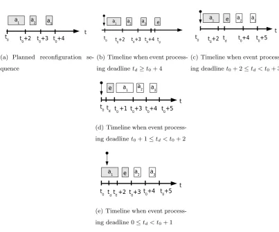
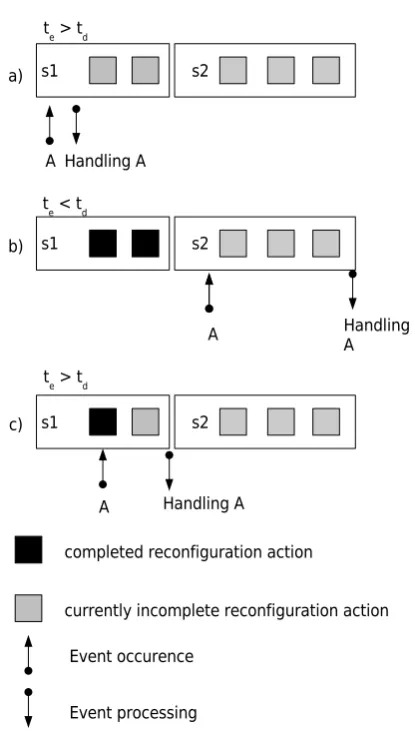
deadline. Figure 1.1 illustrates the basic principle of the time-adaptive execution model by means of a reconfiguration sequence comprised of three reconfiguration actions a1,

a2,a3, which are to be executed sequentially. a1 takes 2 time units to execute, whereas

a2, and a3 take 1 time unit to execute (see Figure 1.1(a)). td denotes the processing deadline of an incoming event, i.e., the maximum time span, until when an event must be processed. Figure 1.1(b) illustrates the case when an event occurs before any recon-figuration action is executed, and with a processing deadlinetd, which is larger than the overall reconfiguration sequence execution duration. In this case all actions can be exe-cuted, before the event is processed. Figure 1.1(c) illustrates the case, where the event also occurs before any reconfiguration action is executed, however, its processing dead-linetdcan only fit the first reconfiguration action. Hence, the remaining reconfiguration actions are executed only, after the event has been processed. Figure 1.1(d) illustrates the case, where even though the event occurs before any reconfiguration action is exe-cuted, the event processing deadlinetdis too small so that no reconfiguration action fits the deadline. Hence, the event is directly processed and the reconfiguration actions are executed after the event has been processed. Case e) illustrates the case when an event deadline is missed and is described in more detail below.

(29)

(a) Planned reconfiguration

se-quence

(b) Timeline when event

process-ing deadlinetd≥t0+ 4

(c) Timeline when event

process-ing deadlinet0+ 2≤td< t0+ 3

(d) Timeline when event

process-ing deadlinet0+ 1≤td< t0+ 2

(e) Timeline when event

[image:29.595.113.517.120.455.2]

process-ing deadline 0≤td< t0+ 1

Fig. 1.1: Execution of reconfiguration actions depending on event processing deadline

td

an incoming event occurs during an executing reconfiguration actiona1. TimeAdapt

(30)

is not met, the software is functioning and can use the data for processing.

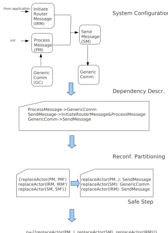
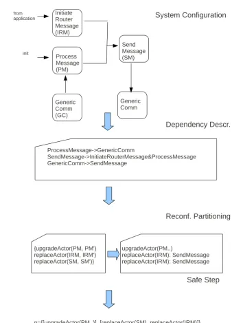
A reconfiguration in TimeAdapt is divided into two phases: a partitioning phase and a scheduling and execution phase. In the partitioning phase, all reconfiguration actions are logically mapped to sub-sequences. The dependency relationship of the software enti-ties, contained in the reconfiguration actions, determines the size of these sub-sequences. The partitioning phase occurs at reconfiguration design time. The scheduling and execu-tion phase takes place at reconfiguraexecu-tion runtime, whenever an incoming event coincides with an ongoing reconfiguration. A scheduling algorithm then decides, based on the available deadline and the estimated reconfiguration action times, how many of the re-maining reconfiguration actions, now logically mapped to sub-sequences, can still be executed before an incoming event’s processing deadline is reached.

(31)

1.4 Contributions

The reconfiguration model described in this thesis contributes to the state of the art in the area of reconfiguration models for software deployed on reactive embedded systems in the following points:

• The dynamic approach towards reconfiguration execution allows the interruption of an ongoing reconfiguration to events that coincide with a reconfiguration. The partial execution of a reconfiguration allows the meeting of processing deadlines, given that the execution duration of the sub-sequence fits within the deadline.

• While supporting incoming events, the reconfiguration approach provides schedul-ing algorithms that execute as many reconfiguration actions as are possible within an incoming event’s deadline, leading to an eventual completion of the reconfigu-ration.

• The reconfiguration model in this thesis supports stateless and stateful software en-tities, and its definition for an abstract, implementation-independent system model allows the application of the model for embedded software in various application domains.

(32)

1.5 Scope

The term “reconfiguration” is often used for the change and optimisation of hardware parts such as FPGA’s (Ghiasi et al., 2005). However, the techniques and mechanisms differ strongly from the ones used in this thesis.

This thesis focusses on the actual process of reconfiguration execution. It is assumed that a reconfiguration sequence is given as input. The procedures for obtaining a re-configuration sequence are beyond the scope of this work. It should also be noted that this work assumes that reconfigurations are valid and do not harm system consistency. Moreover, the issues of trust and security are not covered, i.e., it is assumed that recon-figurations are always for the improvement of the software and not of malicious nature.

1.6 Thesis Outline

The remainder of this thesis is organised as follows. Chapter 2 presents the state of the art in dynamic reconfiguration approaches targeting a variety of embedded software, with a particular emphasis on existing reconfiguration systems and their associated execution models. Chapter 3 presents the design of TimeAdapt and its system model. Chapter 4 presents the implementation of TimeAdapt and the mapping of the system model entities to entities of a component model implementation. Chapter 5 experimentally validates the properties of the reconfiguration model presented in Chapter 3, for software deployed on a real embedded system platform. Chapter 6 summarises and discusses future work.

1.7 Summary

(33)

(34)

Chapter 2

Dynamic Reconfiguration of

Embedded Software

This chapter provides an overview of basic concepts found in dynamic software recon-figuration targeting embedded software in general. Based on this discussion a set of features for reconfiguration models in this domain are derived. This set of features is then used as a guide to review existing reconfiguration models targeting different kinds of embedded software.

2.1 Dynamic Software Reconfiguration of Embedded

Soft-ware

(35)

2.1.1 Dynamic Software Reconfiguration Rationale

Static configuration is commonly applied to embedded software, which is executed on platforms that allow a variety of parameters. Static configuration is defined, according to Perrson (2009), as “the possibility to easily change the configuration of a system at design time through tools.” For example, the features in an automotive control system software, can be personalised according to a customer’s requirements. Static configura-tion has been facilitated by the development of modularised software entities, so-called components, that constitute the embedded software and which allow the modularisation of functionality into different building blocks (Stewart & Khosla, 1996).

The growing complexity of embedded software extends the requirements for config-uration towards reconfigconfig-uration of the software at runtime. There are two rationales for dynamic software reconfiguration. The first one is to handle software failure. A failure occurs when the software is either not functioning or only partially functioning. This includes approaches to formally specify a reconfigurable system that maintains a set of properties when software fails (Strunk & Knight, 2004), to model adaptive embedded software behaviour that can be statically verified (Trapp et al., 2007), and to provide frameworks that realise dynamic reconfiguration when there are faults in the system (Seto et al., 1998).

(36)

2.1.2 Reconfiguration Management

A reconfiguration model defines the possible reconfiguration operations for software en-tities of a specific granularity. A prominent reconfiguration model, which has influenced the subsequent work of many other reconfiguration models, including those targeting embedded software, is Kramer and Magee’s (Kramer & Magee, 1985). This model exe-cutes incremental modifications and is defined for an abstract system model, in which the system is seen as a directed graph with nodes as components and transactions between nodes denoting the connections. A centralised entity, the reconfiguration manager, has a global view on the system and allows the coordination, ordering, and management of reconfiguration actions. The centralised entity sends reconfiguration commands to the respective system entities, which then execute the actual modifications.

In domains, such as peer-to-peer networks or autonomic distributed systems that might involve the adaptation of a large number of software entities, centralised reconfig-uration management might not scale well. These domains need decentralised reconfigu-ration approaches, such as the K-Component approach (Dowling, 2004). In decentralised reconfiguration, the distributed software entities decide, which reconfiguration actions to execute and how to execute them, so-called self-configuration. In contrast to dynamic reconfiguration, self-configuration needs additional algorithms and techniques, such as monitoring, to enable the software entities to detect when and how to execute their own changes. Self-configurable systems are a subset of reconfigurable systems, but are not explicitly dealt with in this thesis. As this thesis deals with non-distributed embedded systems, we adopt the view of a centralised entity that executes reconfigurations.

(37)

and ensure that these reconfigurations are executed in a safe and valid manner. For example, a multimedia conferencing application, comprised of inter-connected devices, might adapt to a different level of network bandwidth. Data must be encoded differ-ently when the level of available network bandwidth decreases. A reconfiguration may involve the replacement of existing encoding filters on the source node, which hosts the streaming application. In this scenario, all receiver devices must replace their decoding filter components to ensure that the communication is not interrupted (Grace, 2008). The entity responsible for the coordination depends on the type of reconfiguration man-agement applied. When using a centralised reconfiguration manager, the coordination is executed as part of this manager.

2.1.3 Reconfiguration Execution

(38)

met, it is not further considered for this thesis.

Kramer and Magee introduced the concept of quiescence as a condition for consis-tency and described mechanisms for how to achieve quiescence by explicitly freezing affected entities (Kramer & Magee, 1990). Once the software is in a quiescent state, reconfigurations can be safely executed, by sequentially executing the remaining recon-figuration actions.

Fig. 2.1: Timing analysis of reconfiguration process (Rasche & Polze, 2003)

While a software entity is in a quiescent state, it cannot process any computations. This is termed the blackout time of a reconfiguration (Schneider et al., 2004). As a high blackout time leads to a high system disturbance, research on dynamic reconfiguration branched into two directions (Li, 2009). One direction focusses on minimising the number of affected entities. For example, Wermelinger extended Kramer and Magee’s approach to block only connections between affected entities (Wermelinger, 1997). Vandewoude relaxed Kramer and Magee’s consistency approach even further by blocking only the affected software entities and not entities that could potentially initiate transactions on these entities, resulting in a very small blackout time (Vandewoude, 2007).

(39)

configuration (Li, 2009). The reconfiguration model then switches, at some point in time, directly between these two configurations, when there are no ongoing transactions for the old configuration. This approach needs additional mechanisms such as transac-tion versioning to determine when the old configuratransac-tion does not process any requests and can be removed safely (Zhao & Li, 2007b).

Reconfiguration Execution Models How a reconfiguration is executed depends

on the actual scheduling approach that is used in the underlying operating system. For example, a preemptive scheduling mechanism associates incoming events with a higher priority and leads to a preemptive execution model. The pre-condition for these models is that the reconfiguration can be directly switched with functional code, without destroying consistency. To achieve this, preemptive reconfiguration models often apply transitional reconfiguration, in which the old and the new configuration are concurrently present. A clock-driven scheduling mechanism either executes the reconfiguration or the functional code of the software, which leads to a transactional execution model. In this execution model a sequence of reconfiguration actions can only be interrupted by events that are known at system design time. Reconfiguration models that follow a transactional execution model are from now on denoted as transactional reconfiguration models, whereas reconfiguration models that follow a preemptive execution model are denoted as preemptive reconfiguration models.

(40)

Requirement/Exec. Model Transactional Preemptive

Guaranteed Reconf. Completion 4 8

Timely Event Response 8 4

Table 2.1: Properties of execution models

To guarantee reconfiguration completion, a preemptive execution model needs to overcome the issue of reconfiguration starvation when there is a high event arrival rate. Possible solutions include the interruption of a reconfiguration only to statically known events (Stewart et al., 1997), or by placing various priorities on incoming events, e.g., used by the preemptive scheduling mode of Zhao & Li (2007b). In the first approach, a reconfiguration preempts only events that are known at system design time. A re-configuration can then be rejected directly, if the rate of these events exceeds a certain threshold. However, reactive embedded systems are exposed to many dynamic event sources, which emit unknown events at arbitrary times. In the second approach, incom-ing events are prioritised accordincom-ing to a given scheme. The reconfiguration model then only interrupts the ongoing reconfiguration to events of a certain priority. However, this approach assumes a specific system model in which events can be tagged and cannot be applied in more general scenarios.

A transactional reconfiguration model meets an incoming event’s response deadline only if the remaining reconfiguration sequence can be completed within this deadline. Before a reconfiguration sequence is started, all events, as well as their arrival rates and deadlines must be statically known, to guarantee that their event deadlines are met (Rasche & Polze, 2005). However, this is not feasible in reactive embedded systems due to the vast occurrence of potential event sources (Regehr, 2008).

(41)

presence of a high event arrival rate, through an incremental execution of remaining reconfiguration actions. We define this kind of execution model time-adaptive, as the execution of the reconfiguration is adapted to its available time, which is constrained by incoming events. In the next section, a minimum set of features is derived that a reconfiguration model should provide in order to enable the timely reaction to incoming events and to guarantee an eventual reconfiguration completion. This set of features is then used to review to what degree existing reconfiguration models for embedded software fulfil the characteristics of a time-adaptive reconfiguration model.

2.1.4 Reconfiguration Execution Models in Hard Real-Time Systems

For completion, we briefly discuss reconfiguration execution in hard real-time systems, and why these models cannot be applied in the kind of embedded software that is considered for this thesis.

Hard real-time systems have additional timing constraints besides their functional requirements, which usually specify that a given activity must be completed within a deadline (Kopetz, 1997). In contrast to the systems we target in this thesis, deadlines in hard real-time systems are strict, and must not be missed. Multi-moded real-time applications are comprised of various operating modes, which each consist of tasks that execute a specific system functionality. For example, a fault recovery mode consists of recovery actions and re-initialisation activities for faulty tasks.

These systems realise dynamic reconfiguration via mode-changes, when there are changes in the environment or changes in the internal state of the application. A mode change removes tasks that belong to the old mode and releasing tasks that belong to the new mode. In a transitioning phase, old tasks are still active and new tasks are scheduled into the system. To guarantee that all tasks reach their deadlines, mode-change protocols are used that differ as to when to delete old tasks and when to schedule new tasks for execution (Real & Crespo, 2004).

(42)

well as their arrival rates and deadlines are known statically before system runtime. In contrast, this thesis considers systems, in which events from unknown sources can occur at arbitrary event arrival rates and have arbitrary associated deadlines.

2.2 Features of a Time-Adaptive Reconfiguration Model

for Embedded Software

Based on the previous discussion, this section lists the characteristics of reconfigura-tion models targeting embedded software. These characteristics can be divided into characteristics that deal with the underlying system model, characteristics of the recon-figuration model itself, and characteristics of the execution model.

2.2.1 System Model Characteristics

Reconfiguration models targeting embedded software can be categorised as system-specific, domain-system-specific, or generic (Zhao & Li, 2007a).

System-specific reconfiguration models target software that is strongly tied to the design of the system it is executed on. This specificity of the underlying software enables the model to make assumptions about the software being changed and to manage change in a way that is optimised for a particular system (Hillman & Warren, 2004).

(43)

Generic system models target software that can be applied in multiple application domains and a wide range of systems. Examples of generic component models include OpenCom (Coulson et al., 2008), and Think (Polakovic et al., 2006). A characteristics of these system models is that they are defined abstractly, in terms of components and connections between components. Different implementations then map these abstrac-tions to actual systems. The abstract definition supports building composable software, independent of the target system or application. The advantage of a reconfiguration model targeting this kind of software is that it is independent of the actual embedded system used.

2.2.2 Reconfiguration Model Characteristics

Reconfiguration model features include correctness guarantees, the point in time when reconfigurations may be triggered, and the constraints on the number of reconfiguration actions and reconfigurable software entities.

(44)

transi-tional reconfiguration that maintains the old and new system configuration in parallel, see Section 2.1.3. Maintaining state invariants is achieved by transferring state between the old and the new software entity.

Reconfiguration approaches differ in whether a reconfiguration is directly executed when it is triggered, or whether it is executed in a delayed fashion, after some other activity has finished completion. Moreover, approaches differ in whether they support an arbitrary number of entities to be reconfigured, for example by supporting the integration of previously unknown software entities, or whether they put constraints on the number of entities to be reconfigured.

2.2.3 Execution Model Characteristics

A reconfiguration that is correct and fulfils a system’s constraints must reach a consistent state by either completing all its actions eventually or by undoing some of the actions, already executed. Depending on its associated execution model, reconfiguration models either react to incoming events that occur arbitrarily, and process them within their deadline, or do not consider incoming events at all.

2.2.4 Summary

This section summarises the set of characteristics of reconfiguration models targeting embedded software, and their possible values. The values, which are most likely to suit a time-adaptive reconfiguration model are shown in bold. Based on this, a set of characteristics for a time-adaptive reconfiguration model is derived.

• System Model

– Entities: system-specific, domain-specific,general

• Reconfiguration Model

(45)

– System correctness: quiescent state,transitional approach

– Possible number of entities to be reconfigured: constrained,unconstrained

• Reconfiguration Execution Model

– Guaranteed reconfiguration completion: Supported due to transactional

execution model, not supported

– React to previously unknown incoming events: Supported due to

preemp-tive execution model, only supported for known events, not supported

These characteristics lead to the following set of required features for a time-adaptive reconfiguration model:

• System Model

F1) The reconfiguration model is defined for a system model suitable for repre-senting embedded software.

• Reconfiguration Model

F2) A reconfiguration can be triggered at any time and there is no a-priori knowl-edge of the possible components that are to be reconfigured in the system. F3) The reconfiguration model does not destroy system correctness.

F4) The reconfiguration model itself does not impose constraints on the reconfig-urable entities.

F5) There are no restrictions on the number of components to be reconfigured.

• Reconfiguration Execution Model

F6) An ongoing reconfiguration is to be completed.

(46)

F8) The reconfiguration model meets an incoming event’s processing deadline.

These features are used in the next section to review existing reconfiguration models targeting different kinds of embedded software.

2.3 Review of Existing Reconfiguration Models

This section presents detailed reviews of reconfiguration models that target different types of embedded software, such as operating system, embedded application, and mid-dleware software. The reviews focus on the degree to which the reconfiguration models represent the features of a time-adaptive reconfiguration model. In all of these models, reconfigurations are triggered for adaptation or evolution purposes and a central entity running on a single processor platform executes the reconfiguration sequence on the un-derlying software entities. Although the domain of addressed software is a super-set of the kind of software addressed in this thesis, the models include a representative sample of the techniques used to reconfigure embedded software that influenced the design of TimeAdapt.

2.3.1 Runes

(47)

System Model The Runes middleware platform is component-based and encapsulates its functionality behind interfaces. The overall architecture follows a two-layer approach. The first layer comprises the basic middleware kernel that provides an API, which allows the dynamic instantiation and registration of components. The second layer comprises components that encapsulate the basic functionalities of applications and middleware services, such as measurement data collection and dissemination components on sensor nodes or publish-subscribe infrastructures on more powerful devices such as laptops.

The component model defines the general architecture of its components in an im-plementation-independent way in terms of the OMG’s Interface Definition Language (IDL) (Object Management Group, 1999). The abstract definition of the component model allows the deployment of components on a variety of system platforms, for which implementations of the system model exist.

Reconfiguration Model The dynamic reconfiguration model is a direct

implementa-tion of Kramer and Magee’s reconfiguraimplementa-tion model with components as the underlying software entities to be reconfigured. The representation of the current system con-figuration as a system graph is realised by using an approach based on architectural reflection (Cazzola et al., 1998). The component model provides an architectural topol-ogy of currently installed and connected software components and interfaces describing operations to inspect and change the self-representation (also known as meta-object pro-tocol (MOP)). Different MOPs reconfigure different parts of the components and their configuration. An architectural MOP allows the structural change of a component’s composition at runtime and an interception MOP allows the behavioural adaptation of a component by introducing interceptors that can add additional behaviour. The mid-dleware kernel represents the central configuration manager that manages and executes the reconfiguration actions on the different components.

(48)

more complex algorithms that support cyclic connections between components (Rasche & Polze, 2008). Reconfiguration actions are then incrementally executed.

The reconfiguration model itself does not put constraints on the number of reconfig-uration actions. It also does not put any constraints on the entities to be reconfigured or the point in time when a reconfiguration may be requested.

Execution Model The reconfiguration execution follows a transactional

reconfigu-ration model. Reconfigureconfigu-ration actions are executed in an uninterruptable manner and the model does not support the interruption of an ongoing reconfiguration for incoming events.

Summary Table 2.2 summarises the features of the Rune’s reconfiguration model.

As can be seen from the table, the Runes reconfiguration model does not allow the immediate processing of incoming events.

Feature System Model (F1) F2 F3 F4 F5 F6 F7 F8

Generic 4 4 4 4 4 8 8

Table 2.2: Features of Runes reconfiguration model

2.3.2 Think

Think is an implementation of the Fractal component model targeting component-based operating systems (Polakovic et al., 2006). The approach tries to improve on existing work for reconfigurable operating system software by loosening the dependence between the reconfiguration model and the underlying platform on which the model is executed.

System Model Fractal defines a hierarchical, reflective component model. It is

(49)

1999). The generic system model supports the application of the reconfiguration model to many operating system platforms. The component model distinguishes two kinds of components. Primitive components can be seen as blackboxes, providing and re-quiring functionality through their interfaces. Composite components are composed of other components, either primitive or composite components. Each component logically comprises two parts, an internal part that implements the functional interfaces of the component and an encapsulating membrane that contains an arbitrary number of control interfaces. Control interfaces provide reflection capabilities such as the manipulation of a component’s interfaces.

Reconfiguration Model Like Runes, Think’s dynamic reconfiguration model is a

direct implementation of Kramer and Magee’s, with software components as the un-derlying reconfigurable entities. Reconfiguration actions in the Think model are either introspection operations, such as the reflective lookup of component interfaces, or inter-cession operations, such as the actual modification of the system. Reconfigurations can either be expressed directly at the level of reconfiguration primitives, provided by the Fractal API, or by using a higher-level domain-specific language such as FScript (David & Ledoux, 2006b).

The Think reconfiguration model is based on quiescence to achieve mutually consis-tent states. This is achieved using approaches such as thread counting or using dynamic interceptors (Polakovic et al., 2006). Reconfigurations are then sequentially executed by the root composite component, which acts as a centralised reconfiguration manager.

Execution Model The reconfiguration execution model is transactional, which

(50)

Summary Table 2.3 summarises the features of Think’s reconfiguration model. Like Runes, the reconfiguration model does not allow the direct processing of incoming events and does not guarantee that an event’s deadline is met.

Generic 4 4 4 4 4 8 8

Table 2.3: Features of Think reconfiguration model

2.3.3 DynamicCon

DynamicCon extends the OSA+ middleware to support dynamic reconfiguration (Schnei-der, 2004). The OSA+ middleware is a middleware system for distributed, real-time em-bedded systems with limited memory and computational resources (Brinkschulte et al., 2000).

System Model OSA+ is a service-based middleware, with a service as the unit of

reconfiguration. A service is an active entity in the middleware and can be comprised of multiple objects. Services have individual control flows to perform application or system tasks and communicate with each other by exchanging jobs. The execution of services is scheduled according to the priorities or deadlines of their corresponding jobs.

Reconfiguration Model DynamicCon has two reconfiguration action types: those

(51)

the reconfiguration service, which then handles all reconfiguration related issues such as plugging in the new service, transferring state from the old service to the new service, and deleting the old service.

In contrast to the previously discussed reconfiguration models, DynamicCon applies a transitional approach to guarantee correctness. The new service is loaded, while the old service can still process requests. A switch between the old and the new service is executed when the complete state has been transferred between the two (stateful) services. One of the main goals of the reconfiguration model is to minimise the blackout time in which a service that is currently reconfigured is unavailable. The model supports different reconfiguration approaches that have different blackout time durations. In the

full blocking approach, the new service is blocked until the old service explicitly calls the switch statement to initiate the exchange of both services. After the switch is executed, the state is transferred. This causes the longest blackout time but at the same time ensures consistent and identical state information on both sides. In the non-blocking approach, the new service version starts to transfer state. During reconfiguration, if the remaining state between the old and the new service can be transferred during this requested blackout time, the reconfiguration is executed completely and all new incoming jobs are processed by the new service. Otherwise, if the requested blackout time cannot be met, the reconfiguration is interrupted and the reconfiguration service keeps monitoring changes to the service state. Incoming jobs are then processed by the old service. Figure 2.2 illustrates this principle.

Execution Model The reconfiguration model takes a transactional view on

(52)

Fig. 2.2: The non-blocking reconfiguration approach (Schneider, 2004)

an event, its response deadline will be met only if it is larger than the requested blackout time.

Summary Table 2.4 summarises the features of DynamicCon’s reconfiguration model.

The constraints on the start time of a reconfiguration and the constraints on support for incoming events makes this reconfiguration model not the ideal candidate for realising a time-adaptive reconfiguration model.

System-specific 8 4 4 4 4 8 8

Table 2.4: Features of DynamicCon reconfiguration model

2.3.4 DynaQoS-RDF

(53)

reconfiguration model has no application disruption time because instead of waiting until a reconfiguration-safe state is reached, the model maintains the old and the new system configuration in parallel.

System Model The reconfiguration model is defined on an abstract system model

that follows a dataflow-driven computational model, the reconfigurable dataflow system model (RDF) (Li, 2009). It allows the modelling of a wide range of embedded software, such as signal processing software, linear and non-linear control system software, and image processing software. The system model extends the concept of a dataflow process network with reconfiguration capabilities of its basic elements, such as processes, data-stores and data-paths (Lee et al., 2003). A process is a computational entity that consumes data through its input ports, processes them, and produces results through its output ports. A data-store holds a specific amount of data, whereas a data-path connects a process with a data-store. Two processes communicate indirectly with each other via their connected data-store.

Reconfiguration Model The reconfiguration model supports the addition and

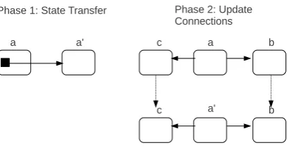
re-moval of processes and data-stores, as well as the addition and rere-moval of data-paths. The model follows a transitional approach to realise consistent system transformations. A dynamic reconfiguration in this model is divided into three phases. Phase one es-tablishes the new configuration. In this phase, software entities, which were previously not installed, are loaded into memory. New incoming data uses this new configuration. Phase two handles switching between the old and the new configuration. Switching includes the completion of data processing by system entities that are part of the old configuration, and starting the processing of new data items only by entities that are part of the new configuration. Phase three removes all software entities that are no longer in use.

(54)

solved by the reconfiguration model, such as guaranteeing transactional non-interleaving and transactional completeness. A transaction is a logical concept that refers to the processing of a requested data-item until the corresponding result is generated. Trans-actions comprise multiple processes and their connections via data-paths. Transactional interleaving occurs if transactions that belong to different configurations interfere. The reconfiguration model avoids these interleavings by applying a version control mecha-nism that isolates data flows belonging to different configurations. Every data-item is assigned a version tag and a process can decide to process this data-item, based on its version number. Transactional completeness means that a transaction, once started, should be completed. This is particularly important during the shutdown period, so that all transactions using processes or data-stores to be removed, are completed. Transac-tional completeness is supported by the underlying system model, in the form of syn-chronisation mechanisms and a tracing mechanism that makes sure that a processor or data-store/path is not currently used so that it can be removed safely.

A reconfiguration can be requested at any given time, and the model supports the introduction of previously unknown software entities and the reconfiguration of an ar-bitrary number of software entities. This puts constraints on the actual entities to be reconfigured. As a pre-condition, each reconfiguration must be directly interruptible. This means that the reconfiguration model does not support reconfiguration actions that will last for a period of time and have an influence on the actual system configuration, such as state transfer. Hence, only stateless software entities are supported.

Execution Model The reconfiguration execution model can be classified as

(55)

Summary Table 2.5 summarises the features of the DynaQoS-RDF reconfiguration model. The reconfiguration model has some intrinsic features of a time-adaptive recon-figuration model, namely its execution model allows the reaction to arbitrary incoming events. However, in the case of many incoming events, the completion of a reconfigura-tion cannot be guaranteed. Also, the model itself imposes constraints on the reconfig-urable entities, such as only the support of stateless software entities.

Generic 4 4 8 4 8 4 4

Table 2.5: Features of DynaQoS-RDF reconfiguration model

2.3.5 Djinn

Djinn is a programming framework, which supports the construction and dynamic re-configuration of distributed multimedia applications targeting embedded systems, such as digital television production, security, and medical systems (Mitchell et al., 1999).

System Model The Djinn system model is generic. Similar to the RDF system model,

(56)

[image:56.595.131.424.436.646.2]

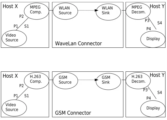
Reconfiguration Model Reconfigurations can be required at any point in time, even though it depends on the actual scheduling time as to when a reconfiguration action will manifest itself in the system. Reconfigurations are executed at the model component layer, with their effects made visible at the peer layer when a reconfiguration is suc-cessfully completed. The execution of the reconfiguration on the model level allows the system to validate the reconfigurations with regards to structural and data constraints. A reconfiguration is expressed in terms of paths. A path encapsulates a group of ports and active components that carry its data. Associated with each path are QoS prop-erties such as latency, jitter and error rate. A reconfiguration will always replace an entire path or sub-path with a new one and has actions such as creating a new active component, deleting active components, and switching input and output ports to the respective active component to use. Figure 2.3 illustrates a reconfiguration example, in which a single video unit is reconfigured to use dial up GSM links instead of local WLan links.

Fig. 2.3: Reconfiguration of a single mobile unit to different communication

(57)

Reconfiguration consistency is achieved by using a transitional approach, i.e., switch-ing between the old and the new configuration. One of the main challenges is mainte-nance of temporal properties during reconfiguration, such as the maximum arrival rate allowed between two data items. Meeting these properties requires reconfiguration ac-tion scheduling. The scheduling algorithm determines when to send events that trigger the activation of a reconfiguration action, so that temporal properties are not violated. To avoid a startup delay for newly integrated components, the reconfiguration is di-vided into two phases, namely a setup and an integration phase. In the setup phase, constraints on the new configuration are checked and new peer components are created as well as resources reserved. The integration phase completes the transition to the final configuration by applying the computed schedule. As illustrated in Figure 2.3, this means that the start event, received by input port P2’ of the H.263 component, needs to be injected before the stop event, received by input port P2 of the MPEG compression component, is sent. This schedule ensures that frames arrive simultaneously at the input port P4 of the display component.

Execution Model The reconfiguration execution model is transactional. This implies

that if not all of the required reconfiguration actions can be scheduled successfully, then none of the actions will be performed and the application will remain in its initial state. The main aim of the model is to maintain application timeliness properties during recon-figuration. The processing of incoming events during a reconfiguration is not supported and a timely response to their deadline not ensured.

Summary Table 2.6 summarises the features of the reconfiguration model. Djinn

(58)

Generic 8 4 4 4 4 8 8

Table 2.6: Features of Djinn reconfiguration model

2.3.6 Port-based Objects

The Port-based Object (PBO) abstraction supports the design and implementation of dynamically reconfigurable real-time control software (Stewart & Khosla, 1996), which can be executed in single and multiprocessor environment. Unlike the previously dis-cussed reconfiguration models, dynamic reconfiguration in this model refers not to the structural change of the system topology but rather switching on and off software entities as part of the current configuration.

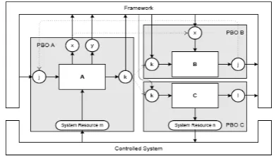
System Model Properties A PBO is an independent concurrent process, which

[image:58.595.182.378.546.657.2]

communicates with other PBOs only indirectly through its input and output ports. Figure 2.4 illustrates three PBOs A, B and C with input and output ports. The output port j of PBO B is connected with the input port j of PBO A, the output port k of PBO A is connected to input port k of PBO B and C. The output port l of PBO C is not connected to any PBO. This loosely coupled infrastructure allows easy replacement of PBOs and makes them the unit of reconfiguration.

(59)

The framework is executed on a controlled system environment, the Chimera RTOS, that provides well-defined communication and memory mechanisms (Stewart et al., 1992).

Reconfiguration Model The dynamic reconfiguration model is strongly tied to the

underlying system model, making it a system-specific reconfiguration model. In contrast to structural changes, which change the topology of the current software, and implemen-tation changes, which change the internals of a software entity, this reconfiguration model changes only the system state of PBOs. All PBOs that are in the ON state denote the currently active configuration. A reconfiguration transforms the currently active config-uration to a new active configconfig-uration. All PBOs that are part of the new configconfig-uration and that are in the OFF state are transformed to theON state and vice-versa.

The reconfiguration steps themselves are executed in idle times of the framework scheduler, i.e., when no PBO is currently executing. An executing PBO is always exe-cuted until its completion so that there is no need for a mechanism to explicitly drive the PBOs into a reconfiguration-safe state.

The model imposes constraints on the number of entities to reconfigure, as it can switch a maximum of nentities, withn denoting the maximum configuration. Entities must be realised by the underlying framework that imposes constraints on those to be reconfigured. Also, switching requires that all modules, potentially required in some con-figuration, need to be known beforehand. This excludes the integration of new software modules downloaded from other systems or the environment after system startup.

Execution Model The reconfiguration execution model follows the preemptive

(60)

time. Because PBOs are scheduled statically, worst-case execution durations for a re-configuration can be calculated. The rere-configuration timetr is the sum of the duration of setting the off and on methods of affected PBOS, the duration of setting up output ports, and the duration of PBOs that interrupt the reconfiguration due to their higher priority. Static scheduling does, however, guarantees reconfiguration completion.

Summary Table 2.7 summarises the features of the PBO reconfiguration model.

Be-cause all PBOs are scheduled statically, a reconfiguration cannot be requested at any time, and the number of reconfigurable entities is restricted by the size of the maxi-mum possible configuration of PBOs. PBO’s system model is specific to a platform and imposes restrictions on the entities, as only entities that follow this model can be recon-figured. The reconfiguration model does not react to incoming events that are unknown at system design time. However, the static scheduling of PBOs guarantees eventual reconfiguration completion and the meeting of timeliness requirements of other PBOs.

System-specific 8 4 8 8 4 8 4

Table 2.7: Features of PBO reconfiguration model

2.3.7 Adaptive Reconfiguration Models

(61)

runs, it is executed following a transactional or preemptive execution model. In contrast to these reconfiguration processes, a time-adaptive reconfiguration process that reacts to incoming events needs to be flexible in terms of which reconfiguration actions still to execute, in order to meet the event’s response deadline and to prevent reconfigura-tion starvareconfigura-tion. Such a reconfigurareconfigura-tion process needs dynamic adaptareconfigura-tion based on the current conditions, such as time constraints, and the entities to be reconfigured.

This section describes two adaptive reconfiguration models that target embedded software, such as operating system software and network stack software. The first is called Molecule and it targets resource-constrained sensor operating systems and selects an appropriate linking method of the modules (Yi et al., 2008). The second, NecoMan, is a middleware that supports the dynamic reconfiguration of programmable network services and customises the applied reconfiguration process according to the properties of the current services that are reconfigured (Janssens et al., 2005).

2.3.7.1 Molecule

Molecule is an adaptive reconfiguration model that targets resource-constrained sensor operating systems (Yi et al., 2008).

System Model In Molecule, software entities are managed as modules. Modules