Evaluating Composite EC Operations and their
Applicability to the on-the-fly and Non-Window
Multiplication Methods
Mohammad Rasmi
Zarqa University, Jordan
Hani Mimi
Alzaytoonah University, Jordan
Mohammad Sh. Daoud
Al Ain University of Science and Technology, UAE
ABSTRACT
In order to improve the efficiency of elliptic curve multiplication methods, extended and composite elliptic curve operations such as 𝒏𝑷, 𝒎𝑷 + 𝑸, where 𝒏 > 2and 𝒎 ≥ 𝟐 , and repeated doublings were proposed. These operations have lower complexity, in terms of field operations, than that for classical methods. Moreover, they are supposed to replace the classical methods. In this paper, repeated doublings and odd point computation are deeply analyzed in order to measure their actual efficiency. According to the gained results, the improvement ratio in the execution time is not the same as the improvement ratio measured in terms of field operations. Moreover, different implementations of Sakai repeated doubling method yield different results. For example, implementing 4P as a separate function gives lower complexity than implementing repeated doublings as a general function. On the other hand, other methods for computing nP, where n is odd, have been analyzed. Dahmen method failed to meet the expected results for computing odd points in elliptic curve multiplication methods that employ the on-the-fly strategy since its time complexity was more than that for classical methods. It was also found that new techniques should be devised to improve the efficiency of window methods for calculating odd points such as: 5P, 7P, and 15P, which have lower cost than that for classical method.
Keywords
Repeated doublings, extended elliptic curve operations, pre-computations, single scalar multiplications, recoding methods
1.
INTRODUCTION
Elliptic Curve Cryptography (ECC) was proposed in 80’s of the previous century. The same level of the well-known RSA cryptographic algorithm security can be achieved by smaller key sizes in ECC systems [1]. The performance of ECC schemes is better than that for other public key schemes. Therefore, it is more suitable for devices with limited resources such as personal digital assistants (PDAs) and mobile phones [2]. The hamming weight (𝑘) , which is the ratio of the nonzero digits to the key length, affects the efficiency of elliptic curve (EC) multiplication methods. Other recoding methods such as signed methods were invented in order to reduce the amount of hamming weight, for example the non-adjacent form (NAF) signed binary method were used to accelerate the EC multiplications [3].
Window methods, such as Mutual opposite form (wMOF) [4] and wNAF, were also used in EC multiplications in order to its efficiency. Other recoding schemes were also introduced to improve the efficiency of computing the point 𝑘𝑃,wehre𝑘 ∈
𝐼, 𝑃 ∈ 𝐸(𝐹𝑃) such as multi-base or mixed-base recoding
methods, double base number system (DBNS) [5, 6] is an example.
Computing kP involves two basic EC operations: doubling (2𝑃) and addition (𝑃 + 𝑄). Extended and Composite (simply Composite) EC operations are those other than the basic operations, i.e. 𝑛𝑃, 𝑤𝑒ℎ𝑟𝑒 𝑛 > 2 𝑎𝑛𝑑 𝑚𝑃 + 𝑄, 𝑤ℎ𝑒𝑟𝑒 𝑚 ≥ 2. Recoding methods, such as window and multi-base, involve both types of operations: basic and composite. Therefore, researchers such as Ciet[7], Sakai [8], Dahmen[9], and Eisentrager[10] explored this area and come up with extended and composite EC operations based on Affine and Jacobian, coordinate systems. The cost, in terms of the number of underlying field operations, of these new invented operations is lower than the cost of classical methods.
The EC operations, basic and composite, involve underlying field operation such as inversions (i), multiplications (m), squarings (s), and additions. In large prime fields, additions are neglected and the ratio 𝛽 =𝑚𝑠 is considered 0.8 if the algorithm is not protected against side channel attack (SCA) [11]. If the algorithm is protected against SCA , the same multiplier is used to perform both operations in order to be indistinguishable [12]. The ratio 𝛼 =𝑚𝑖is used to represent the relative cost between field inversion and field multiplication [12, 13].
Up to our knowledge and based on the literature, there is no study that combines the composite EC operations together and takes advantage of these methods or analyzes the actual performance (execution time) of these methods. Thus, the goal of this paper is to measure the actual performance of these methods and find out if the amount of enhancement in the actual performance will meet the expected performance. This paper investigates these methods and analyzes them in order to come up with some recommendations by answering the question: Can these methods really reduce the cost of EC scalar multiplication methods? A feasibility study of exploiting these methods in EC multiplication methods is conducted. The expected performance is measured by calculating the field complexity (FIELD-COMPLEXITY), while the actual performance represents the execution time measured by implementing the algorithm (TIME-COMPLEXITY). The FIELD-COMPLEXITY is defined as the number of underlying field operations required by the EC operations. Inversion operations and squaring are replaced by equivalent multiplication. Thus, FIELED-COMPLEXITY is measured by the total number of required multiplications.
2.
BACKGROUND TEHORY
2.1
Elliptic Curve Arithmetic
A Weierstrass equation is simplified in order to facilitate the usage of elliptic curve equation in elliptic curve cryptography. The following equation is defined over the prime field Fp with characteristic >3.
𝐸: 𝑦2𝑚𝑜𝑑𝑝 = (𝑥3+ 𝑎𝑥 + 𝑏) 𝑚𝑜𝑑𝑝 (1)
Where 𝑎, 𝑏, 𝑥, 𝑦𝐹𝑝and ∆= −16(4𝑎3+ 27𝑏2)
The value of the discriminant ∆ determines if the curve can be used in the elliptic curve cryptosystem. The set of all points on the curve are denoted by 𝐸 𝐹𝑝 while the total number of these
points is denoted by #𝐸 𝐹𝑝 . The identity point ∞is called the point at infinity. The value of the coefficient a in the elliptic curve equation is considered -3 for all NIST (National Institute of Standards and Technology) elliptic curves without much loss of generality [13, 14]. It is known that exponentiation is defined as repeated multiplication, but when we talk about elliptic curve exponentiation or multiplication, it means repeated additions. For example, the value ab is simply calculated by multiplying a by itself b times (i.e. 𝑎𝑏= 𝑎 × 𝑎 × … × 𝑎
𝑏𝑡𝑖𝑚𝑒𝑠
). In elliptic curve
cryptography, the quantity 𝑘𝑃 is simply calculated by adding P to itself k times (i.e. 𝑘𝑃 = 𝑃 + 𝑃 + ⋯ + 𝑃
𝑘𝑡𝑖𝑚𝑒𝑠
).A more elaborated
method called double-and-add which is the counterpart of the square-and-multiply method depends on two basic operations: addition and doubling [1, 15].
Let 𝐺 = (𝑥1, 𝑦1) and 𝑄 = 𝑥2, 𝑦2 where 𝐺 ≠ −𝑄 . Let represents the point at infinity. Then
1. 𝐺 + ∞ = 𝐺
2. 𝐺 + −𝐺 = ∞, where – 𝐺 = ( 𝑥1, −𝑦1)
3. 𝑅 = 𝐺 + 𝑄 = (𝑥3, 𝑦3)
𝑥3= (𝜆2− 𝑥1− 𝑥2) 𝑚𝑜𝑑𝑝
𝑦3= 𝜆 𝑥1− 𝑥3 − 𝑦1 𝑚𝑜𝑑𝑝.
𝜆 =
𝑦𝑥2− 𝑦1
2− 𝑥1 𝑚𝑜𝑑𝑝𝑖𝑓𝐺 ≠ 𝑄
3𝑥12+ 𝑎
2𝑦1 𝑚𝑜𝑑𝑝𝑖𝑓𝐺 = 𝑄
Elliptic curve addition operation needs a total cost of (𝑖 + 2𝑚 +
𝑠) field operations if affine coordinate system is used, where i, m, and s refers to inversion, multiplication, and squaring respectively. Doubling operation needs (𝑖 + 2𝑚 + 2𝑠) field operations. The most expensive operation in prime-field arithmetic is the inversion operation. The cost of inversion is determined by the ratio 𝑚𝑖. This ratio represents the number of multiplications that is equal to one inversion. The ratio 𝑚𝑖 is estimated between 30 and 80 in [11, 13, 16].
2.2
Composite and Extended Elliptic Curve
Operations
Extended and composite (or simply composite) operations are those other than basic EC operations. EC multiplication methods depend on some composite operations in addition to the basic operations. Thus, researchers such as Ciet[7], Guajardo [17], and Sakai [8] proposed composite operations that can be calculated with less cost than that for classical methods. Researches tried to trade inversions for lower cost modular operations such as multiplication and squaring, since modular inversion is the most expensive operation under prime fields.A direct formula for
computing 𝑛𝑃, where n is an integer, was introduced by [18] and [19]. However, these methods were not computationally efficient as stated by [17] for fast 𝑛𝑃 calculation. The first method for computing repeated doublings using only one inversion was introduced by [17] in 1997. They introduced new method to compute 4𝑃, 8𝑃, 𝑎𝑛𝑑 16𝑃 directly using only one inversion for elliptic curves defined over binary fields. The author of [20] succeeded to compute4𝑃 using at most 𝑖 + 14𝑚 + 7𝑠 for elliptic curves defined over prime fields using affine coordinates. On the other hand, direct computation of 4P using projective coordinates over prime fields was proposed by [21]
The idea of reducing the complexity (i.e. increasing the speed) of elliptic curve point multiplication by trading field inversions with multiplication and squaring has been also addressed by other researchers [7, 8, 10]. In [10] the authors proposed a new method for computing 2𝑃 + 𝑄 that saves one field multiplication compared to the classical method. They omitted the y coordinate when calculating 𝑃 + 𝑄 which saves a field multiplication either when 𝑃 = 𝑄 or when 𝑃 ≠ 𝑄. Moreover, the cost of calculating 3𝑃 + 𝑄was reduced using the same trick.
They compared the performance of their formulas with the classical methods over binary and prime fields P160 and P256. They mentioned that the ratio 𝛼 =𝑚𝑖 was 3.8 for P160 and 4.8 for P256. They said that 8.5% saving could be achieved for a window size 1 and 𝛼 = 4.18. The value of 𝛼 that was considered in that paper was estimated without employing Montgomery method, which is faster than the traditional multiplication method. The estimations of other researchers such as in [16]for
𝛼was more accurate. It is considered 𝛼 > 40 while it is considered 80 in [13]. Later on, it is considered between 30 and 50 in [1]. In this study the value of 𝛼 that has been achieved is 22. Therefore, if 𝛼 is considered 100, the saving will be 0.6%, 1.2% for 𝛼 = 50, and 2.3% for 𝛼 = 25.Thus, their theoretical saving, in terms of field operations, is not as expected. Finally, we should highlight that the comparison was theoretical, without implementation. Later on, new methods for computing 2𝑃 +
𝑄, 3𝑃, and 3𝑃 + 𝑄, that are faster than the traditional methods using affine coordinates whenever a field inversion costs more than six multiplications was proposed by [7]. The proposed formulas are also faster than the proposed formulas by [10] whenever 𝛼 > 6. The formula 4𝑃 + 𝑄was mentioned in the paper but without providing the algorithm.
2.3
Repeated Doublings
[image:2.595.66.237.399.527.2]A repeated doubling method was proposed by Sakai and Sakurai [8] using only one inversion in affine and weighted projective coordinates. Their method was more efficient than the method proposed by Muller [20].
Table 1 Complexity Comparison [8]
Calculation
Sakai Classical Break-even point
𝛼 >
m S i m s i
4P 9 9 1 4 4 2 8.6
8P 13 13 1 6 6 3 6.3
16P 17 17 1 8 8 4 5.4
2dP 4d+1 4d+1 1 2d 2d d 3.6𝑑 + 1.8
Sakai and Sakurai computed 2𝑑𝑃, where P is random elliptic curve point, directly without computing the intermediate values
2𝑃, 22𝑃, . . . , 2𝑑−1𝑃 for 𝑑 ≥ 1.Their method is faster than the
classical method in terms of fields operations for𝐸(𝐹𝑝). The
classical method here means separated doublings using the basic EC operation, which is doubling. Table 1 shows the FIELD-COMPLEXITY analysis of their method compared to the classical method. The number of inversions was reduced at the cost of multiplication and squaring.
2.4
Computing Odd Points
A method for reducing the complexity of computing odd points had been proposed by [9]. In order to pre-compute the odd points
3𝑃, 5𝑃, … , [2𝑑 − 1]𝑃 using affine coordinates. Their method is a simultaneous recursive method to reduce the total number of inversions using Montgomery trick [22] p.209. The proposed method pre-computes all odd points 3𝑃, 5𝑃, … , [2𝑑 − 1]𝑃 on elliptic curves defined over prime fields, where the points are represented in affine coordinates, only using one single field inversion for the computations. The cost of this method in terms of underlying field operations is [(10𝑑 – 11)𝑚 + (4𝑑)𝑠 + 𝑖]. There are many methods for computing the inversion in the finite prime field. One method is known as plus-minus method. Another one proposed to compute the inverse if the modulus P is prime. Montgomery also deals with single inverse and simultaneous inversion where j elements a1,…,aj modulo p are to be computed [22].
3.
RESULTS AND ANALYSIS
[image:3.595.305.544.497.618.2]In order to use Elliptic Curves in cryptographic applications, many parameters should be determined first. One of these parameters is the base point P that will be used in the multiplication algorithm [14, 23]. Fortunately, there are 10 recommended ECs defined over binary and prime fields published by the national institute of standards and technology (NIST). The curves used in this research are the NIST recommended curves that are defined over prime fields [13]. In addition, the base point used in our experiments, 𝑃(𝑥, 𝑦), is given with each NIST recommended EC [14]. The parameters of these ECs can be found in FIPS PUB 186-3 [14]. The algorithms used in this research are implemented using the MIRACL cryptographic tool [23] since it supports EC applications over prime fields. It is considered the best tool, among other libraries, for EC operations in windows platform [23, 24].
Table 2 Specifications of the PCs used in the experiments
System Information
Operating
System Processor Memory
PC1
Windows XP Professional
SP3
AMD Quad-Core Processor, MMX,
~2.3GHz
3.6 GB
PC2
Windows XP Professional
SP3
Pentium(R) Dual-Core CPU 2.00GHz (2 CPUs)
3 GB
In this paper, affine coordinates for curves defined over Fpwere considered. Several experiments, using two different PCs, have been conducted over hundreds of thousands of randomly chosen n bit keys, where 𝑛 ∈ {160, 192, 224, 256, 384, 521} . Computers’ specifications are summarized inTable 2. The value of 𝛼 is estimated by 22, and the ratio 𝛽 =𝑚𝑠 is estimated by one. In the following sections, the introduced algorithms are analyzed and compared to the classical methods.
3.1
Repeated Versus Classical Doubling
The time complexity and field complexity should be analyzed for Sakai method [8]compared to classical method. As mentioned earlier, Sakai method computes the repeated doublings of the form 2𝑑𝑃 𝑓𝑜𝑟 𝑑 ≥ 1. By referring to Sakai paper [8] and according to Table 3,there was no comparison between their method and classical method in terms of TIME-COMPLEXITY. In other words, they measured the timings of a point addition and direct doublings in milliseconds without comparing their results with separated doublings. For example, there is no comparison between 2P-Sakai and 2P-Classical, 4P-Sakai and 4P-Classical, and so on. On the other hand, they implemented their method with w-NAF (window NAF) where
𝑤 = 2,4 and then compared the resutls. They showed a performance improvement because the dominant number of doublings is four, which is 69% of all doublings, as shown in Table 3.
Table 3 Number of computations of 2d, where d=1,2,3, or 4, and additions in the sliding signed binary window method
with window length 2 or 4 [8]
Key size 4-NAF (window size = 4)
2P 4P 8P 16P
160 14.93 4.99 2.58 31.75
192 15.29 5.06 2.64 39.54 224 15.31 5.05 2.69 47.49
256 15.31 5.06 2.7 55.53
384 17.13 5.1 3.59 86.26
521 31.34 14.51 6.94 109.87 Avg. 18.21833 6.628333 3.523333 61.74
Percent 20% 7% 4% 69%
In order to examine the efficiency of Sakai method versus classical method; firstly a theoretical comparison between Sakai and classical method is conducted in terms of FIELD-COMPLEXITY and the results are presented in Table 4.
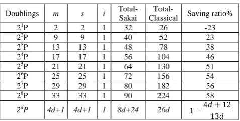
Table 4 Number of field multiplications needed by Sakai and classical methods and the improvement ratio
Doublings m s i Total-Sakai Classical Total- Saving ratio%
21P 2 2 1 32 26 -23
22P 9 9 1 40 52 23
23P 13 13 1 48 78 38
24P 17 17 1 56 104 46
25P 21 21 1 64 130 51
26P 25 25 1 72 156 54
27P 29 29 1 80 182 56
28P 33 33 1 90 224 58
2dP 4d+1 4d+1 1 8d+24 26d 1 −4𝑑 + 12
13𝑑
Sakai method was designed for repeated doublings, therefore it does not improve doubling formula when 𝑑 = 1in 2𝑑𝑃. It is inefficient for single doubling[8]. The last column shows the percent of theoretical reduction compared to classical doubling method. The total number of multiplications needed by Sakai method is 𝛼 + 4𝑑 + 1 + 4𝑑 + 1 𝛽 where the total number of multiplications needed by classical method is 𝑑𝛼 + 2𝑑𝑚 + 2𝑑𝛽. Finally, the saving ratio is generalized to 1 −4𝑑+1213𝑑 .
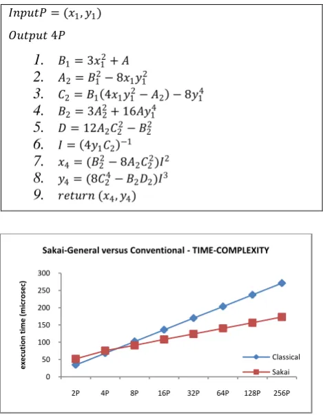
[image:3.595.54.288.559.638.2]the execution time did not meet the expectations especially for computing 4P. In Cietpaper [7], a separate algorithm for computing the quantity 4P is introduced based on Sakai method.The execution time of 4P, when implemented as a separate function, is better than that for classical method. Consequently, two algorithms are considered: general Sakai algorithm (Sakai-General) that computes 2𝑑𝑃, 𝑓𝑜𝑟 𝑑 ≥ 1[8], and Algorithm 1, 4P-Sakai [7] in which the algorithm is only used for computing 4P.
Algorithm 1 4P-Sakai: Calculating 4P for E(Fp)
𝐼𝑛𝑝𝑢𝑡𝑃 = (𝑥1, 𝑦1)
𝑂𝑢𝑡𝑝𝑢𝑡 4𝑃
1.
𝐵1= 3𝑥12+ 𝐴2.
𝐴2= 𝐵12− 8𝑥1𝑦123.
𝐶2= 𝐵1 4𝑥1𝑦12− 𝐴2 − 8𝑦144.
𝐵2= 3𝐴22+ 16𝐴𝑦145.
𝐷 = 12𝐴2𝐶22− 𝐵226.
𝐼 = 4𝑦1𝐶2 −17.
𝑥4= (𝐵22− 8𝐴2𝐶22)𝐼28.
𝑦4= (8𝐶24− 𝐵2𝐷2)𝐼3 [image:4.595.308.538.72.195.2]9.
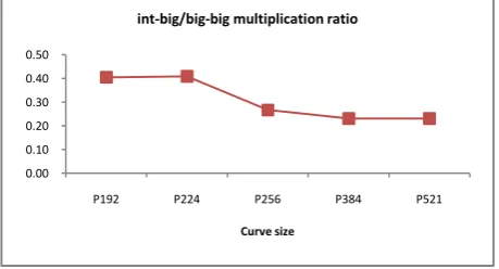
𝑟𝑒𝑡𝑢𝑟𝑛 (𝑥4, 𝑦4)Figure 1 Execution time of Sakai versus classical
Figure 1shows the average execution time resulted from implementing Sakai-General against the classical method over various curve sizes. Each point on the figure represents an average of at least 100,000 experiments. As it can be seen from the figure, Sakai-General method is not useful for single doubling or 2 repeated doublings, i.e. 𝑑 = 1 or 2 in 2𝑑𝑃. On the other hand, it works well when 𝑑 ≥ 3in 2𝑑𝑃. Therefore, we can see that Sakai-General method is useful for theEC multiplication methods that depend on repeated doublings, such as window-based methods, were repeated doublings are the dominant operation.
As a conclusion, we have seen that Sakai-General method did not meet the expectations regarding 4P. Calculating 4P using Sakai methodrequires+9𝑠 + 9𝑚, which is equivalent to 42 multiplications for𝛼 = 22, and 52 multiplications if the classical method is used. Theoretically, Sakai costs 25% less than 4P-Classical, but the implementation of Sakai-General did not reflect this ratio, there was no enhancement at all. This leads us to implement 4P-Sakai using standalone function 4P-Sakai. Anyhow, a performance test has been carried out to compare 4P-Sakai with classical method and the results are shown in Figure 2. Each point represents an average of 300,000 experiments.
Figure 2 Comparing TIME-COMPLEXITY of 4P
[image:4.595.54.289.185.487.2]It is noticed from Figure 2 that the best method to compute 4P is Sakai method. The execution time of computing 4P using 4P-Sakai was the lowest. An improvement of 11% in the performance over all sizes of elliptic curves has been achieved. Therefore, 4P-Sakai should be implemented as a separate (standalone) function. Finally, Table 5 shows the saving ratios in terms of running time and field operations. As it can be seen from the table, the saving ratio when the algorithm is implemented differs from the estimated saving ratio. In general, there is 51% average differencebetween the TIME-COMPLEXITY and FIELD-TIME-COMPLEXITY improvements.
Table 5 Saving ratio of Sakai in terms of field operations and execution time
Doublings
Saving ratio
Difference
FIELD-COMLEXITY
TIME-COMLEXITY
21P -23% -51% 0
22P 23% 8% 67%
23P 38% 11% 72%
24P 46% 20% 56%
25P 51% 27% 47%
26P 54% 31% 42%
27P 56% 34% 39%
28P 58% 36% 37%
3.2
Analyzing Odd Point Computation
A FIELD-COMPLEXITY analysis has been done in order to compare the computation of the points (3P, 5P, 7P, 15P, 21P, and 31P) using Dahmen method [9] against classical method. The gained results are depicted in Figure 3. Recall that the cost of Dahmen method in terms of underlying field operations can be calculated using the formula [(10𝑑– 11)𝑚 + (4𝑑)𝑠 + 𝑖]. On the other hand, the cost of classical method has been calculated using the cost of basic EC operations: additions and subtractions. It is also worth to be mentioned here that the computed field complexity for these operations is independent of the field size. The field size does not count in the calculations that have been done to draw Figure 3.
Figure 3 Comparative analysis of Dahmen method against classical method in terms of number of multiplications 0
50 100 150 200 250 300
2P 4P 8P 16P 32P 64P 128P 256P
e
xecut
ion
t
im
e
(
m
icr
os
e
c)
Sakai-General versus Conventional - TIME-COMPLEXITY
Classical
Sakai
30 50 70 90 110 130
P192 P224 P256 P384 P521
Execut
in
o
ti
m
e
(
m
icr
os
e
c)
Prime field size 4P Comparitive Complexity
classical Sakai-General 4P-Sakai
0 50 100 150 200 250
3P 5P 7P 15P 21P 31P
fi
e
ld
m
u
lt
ip
lica
ti
on
FIELD-COMPLEXITY
[image:4.595.300.550.356.470.2] [image:4.595.307.537.618.726.2]As it can be seen from Figure 3, although Dahmen method depends only on simultaneous inversion (which counted as one inversion by the authors) in the computation, the number of multiplications required by Dahmen method is more than that for the classical method for the points 21P and 31P. While the number of required multiplications by Dahmen method in computing the points 3P, 5P, 7P and 15P is less than that for classical method. It can be concluded that for computing kP, for odd k, Dahmen method loses its improvement whenever k grows. Dahmen method is mainly proposed for precomputations.Nonetheless,Dahmen method will be investigated if it can be used to replace classical method for odd point computations.Thus, a TIME-COMPLEXITY analysis has been done and the results are summarized in Figure 4.
Figure 4 Comparative analysis of Dahmen method against classical method in terms of execution time
By referring to Figure 3 and Figure 4, we can see that although FIELD-COMPLEXITY of Dahmen method is better than that for classical method for computing the points 3P, 5P, and 7P, its TIME-COMPLEXITY is worse than that for classical method. In order to understand this result, a deeper investigation about Dahmen algorithm is carried out. When referring to Dahmen algorithm [9] we can see two types of multiplications. Firstly, small integer multiplied by large integer (it is denoted by intbig) such as 𝑑1= 2𝑦1 where 2 is an integer and y1 is large
integer since it’s the y coordinate of the point P. Secondly, large integer multiplied by large integer (it is denoted by bigbig) such as 𝐵 = 𝐸 ∙ 𝐵 where both are defined as large integers.
The cost of bigbig multiplication is compared with the cost of intbig multiplication. Moreover, anintbig multiplication, where the integer int∈ {2,3, … ,9},could be replaced by addition if the cost of addition is cheaper than the cost of intbig multiplication (for example 2X, where X is a big integer, could be replaced by one addition; X + X). Thus, the efficiency of replacing intbig multiplication by addition is investigated, where intbig means small integer (≤ 10) multiplied by big integer. Finally, Dahmen algorithm uses Montgomery simultaneous inversion trick which is also need to be compared with Montgomery single inversion method [22].
[image:5.595.307.537.341.465.2]In Elliptic curve multiplication algorithms we have two types of multiplications, small integer multiplied by big-integer (intbig) and big-integer multiplied by big-integer (bigbig). Researchers always neglect the cost of additions, subtractions, and intbig multiplications since their cost are low compared to bigbig multiplication, squaring and inversions [4, 12, 25]. Since the theoretical efficiency of Dahmen algorithm is not as the practical efficiency, the previous facts should be reconsidered.
Table 6 Updated complexity of Dahmen method in terms of field multiplications
FIELD-COMPLEXITY Classical Dahmen Dahmen+2
computation m m m
3P 51 39 41
5P 77 53 55
7P 102 67 69
15P 153 123 125
21P 154 165 167
31P 204 235 237
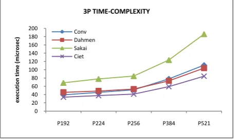
By referring to Dahmen algorithms found in appendix A [9], the number of required intbig multiplications by Dahmen algorithm is 7[9]. The TIME-COMPLEXITY of intbig and bigbig multiplications is shown in Figure 5.
Figure 5 Multiplication ratio of intbig to bigbig
Each point on the figure represents an average of 5 million iterations. As it can be seen from the figure, the cost of intbig multiplication is 0.4 of bigbig multiplication for the curves P192 and P224. The average ratio intbig/bigbigover all curves is 0.31. This means that three intbig multiplications cost as one bigbig multiplication. As mentioned earlier, Dahmen method [9] requires 7 intbig operations. Therefore, their cost will be replaced by two bigbig multiplications. The updated complexity of Dahmen method [9]is depicted in Table 6. For example, after this analysis has been done, the cost of computing 3P is updated from 39𝑚 to 41𝑚 because two multiplications are added.
The next issue that should be determined is the cost of intbig multiplication compared to additions. For example, 2𝑋, where
𝑋 is big integer, can be computed simply by intbig multiplication or using addition, 𝑋 + 𝑋. The results of this study are summarized in Figure 6. Each point on the curve is an average execution time for 𝑎𝑋 where 𝑎 ∈ {2,3,4,5,6,8} and 𝑋 is a big-integer (a point on elliptic curve). It also represents an average of 100,000 experiments. The execution time for both methods does not differ that much over all curves. Therefore, intbig multiplication can still be used, but addition is preferred if the integer number is small.
0 50 100 150 200 250 300 350 400 450 500
3P 5P 7P 15P 21P 31P
e
xecut
ion
t
im
e
(
m
icr
os
e
c)
TIME-COMPLEXITY
Classical
Dahmen
0.00 0.10 0.20 0.30 0.40 0.50
P192 P224 P256 P384 P521
Figure 6 Comparative analysis of computing nP by
multiplication or by addition, where 2 ≤ n ≤ 8 and P∈E(Fp)
[image:6.595.55.295.70.201.2]Finally, since Dahmen method uses Montgomery trick [22]with simultaneous inversion, another comparison is conducted.
Figure 7 Montgomery single inverse running time against Montgomery multi-inverse
Figure 7 shows the results gained from comparing single-inverse method with multi-inverse method over all curves. Each point represents an average of 100,000 experiments. The execution time of single-inverse method is always less than that for multi-inverse method even when the number of simultaneous inversions is two as in 2-inv curve in the figure. Therefore, the complexity of Dahmen method will be higher when the number of simultaneous inversions increases.
As a summary of investigating Dahmen method, which is implemented as in [9], and its applicability to the on-the-fly EC multiplication methods, we saw that the FIELD-COMLEXITY of Dahmen method was better than that for classical method for computing the points {3𝑃, 5𝑃, 7𝑃, 15𝑃}. On the other hand, it gets worse for computing {21𝑃, 31𝑃}; i.e. when d grows in the formula (2𝑑 − 1)𝑃. Despite the FIELD-COMPLEXITY of Dahmen method was lower than that for classical method, Dahmen method is not suitable for computing odd points using on-the-fly EC multiplication methods because of the extra complexity discovered when the method was analyzed. Their method is more suitable for precomputations with window methods. Thus, it is recommended to use classical method rather than Dahmen method for odd point computation of the form
[2𝑘 − 1]𝑃.Enhancing Dahmen method is another solution if possible. Another solution could be achieved by inventing new method that has lower cost than Dahmen method.
3.3
Analyzing 3P Computation
The odd point 3P can be computed using several methods: (1) Dahmen (3P) [9], (2) classical (3𝑃 = 2𝑃 + 𝑃), (3) Ciet (3P) [7], (4) Sakai method using Morain trick (3P = 4P-Sakai – P) [8, 26].
Figure 8 Field complexity of computing 3P using several
methods
Figure 8 shows the number of multiplications needed by all of these methods whenever 𝛼 = 22 𝑎𝑛𝑑 𝛽 = 1. As you can see, Ciet method has the lowest FIELD-COMPLEXITY cost which means that it could be used to compute 3P. In order to make sure that 3P-Ciet is the best method, a TIME-COMPLEXITY analysis should be done to compare these methods.A performance analysis has been done to judge the efficiency of the introduced methods to compute 3P. The results of these experiments over several elliptic curves are summarized in Figure 9. Each point on the figure represents an average of 300,000 iterations. The worst execution time was for 3P-Sakai while the best execution time was for Ciet method. Consequently, 3P-Cietshould be used instead of other methods.
Figure 9 time complexity of computing 3P using several methods
3.4
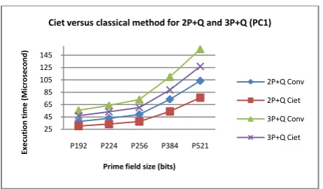
Analyzing 2P+Q and 3P+Q
Two other composite formulas were improved by Ciet[7],
2𝑃 + 𝑄 and 3𝑃 + 𝑄. These formulas are also tested. We compared the expected performance and the actual performance for Ciet method against classical method. The least cost for classical method is to compute 2𝑃 + 𝑄 as (𝑃 + 𝑄) + 𝑃 and for
[image:6.595.55.285.259.390.2]3𝑃 + 𝑄 using three additions as follows:((𝑃 + 𝑄) + 𝑃) + 𝑃.The FIELD-COMPLEXITY for both methods is shown in Table 7.
Table 7 Mathematical Cost Comparison
Operation Classical Ciet
m s i m s i break-even point 2P+Q 4 2 2 9 2 1 5 3P+Q 6 3 3 9 4 2 4
The execution time for both methods is shown in Figure 10. As it can be seen from both figures, Figure 9 and Figure 10, the TIME-COMPLEXITY of Ciet composite formulas is better than that for classical method. Thus, Ciet showed a performance improvement over classical method in both cases TIME-COMPLEXITY and FIELD-TIME-COMPLEXITY.
0.0 0.1 0.2 0.3 0.4 0.5 0.6
P192 P224 P256 P384 P521
e
xecut
ion
t
im
e
(
m
icr
os
e
c)
Curve size TIME-COMPLEXITY
Mult
Add
0 20 40 60 80 100 120 140
P192 P224 P256 P384 P521
e
xecut
ion
t
im
e
(
m
icr
os
e
c)
Curve size
TIME-COMPLEXITY single-inverse against multi-inverse
2-inv
3-inv
5-inv
10-inv
single-inv
3P
33 51 39
65 3P const in terms of field multiplicaions
Ciet conv Dahmen Sakai
0 20 40 60 80 100 120 140 160 180 200
P192 P224 P256 P384 P521
e
xecut
ion
t
im
e
(
m
icr
os
e
c)
3P TIME-COMPLEXITY
[image:6.595.306.536.383.520.2] [image:6.595.323.526.650.703.2]Figure 10 Execution Time Complexity of Ciet versus classical EC Multiplication Methods
4.
CONCLUSION
In this research, among other repeated doubling methods Sakai methodhas been examined. It is found that it has the lowest field complexity.The saving ratio of Sakai compared to classical method in terms of field complexity was generalized to 1 −
4𝑑+12
13𝑑 . According to the conducted experiments,it was found
that Sakai method should be represented in two separate functions; the first one is Sakai-general for computing 2dP where d ≥ 2, and the second one is 4P-Sakai for computing 4P in order to get the full efficiency of the method. Sakai method is more efficient than classical method for EC multiplication techniques that depend on window recoding strategies or multi-base numbering systems. The average difference between the improvement ratio of TIME-COMPLEXITY and FIELD-COMLEXITY is 51%. Consequently,Sakai method improves window-based EC multiplication methods by at least 12−2𝑑+613𝑑 . Other composite EC operations, proposed by Dahmen for the precomputations stage, have been also tested in order to determine if it can improvethe on-the-fly EC multiplication methods.The experiments showed that the efficiency of the classical method is better than that for Dahmen method. The analysis that has been done in this research showed that Dahmen method depends on Montgomery simultaneous inversion technique. They considered it as a single inversion when they analyzed their method. It was found here that Montgomery single inversion technique has a lower cost than Montgomery simultaneous inversion in terms of TIME-COMPLEXITY. Their method has been deeply analyzed and it was found that there was an extra overhead to be added to the complexity of Dahmen method. As a result of the investigations,Dahmen method should not be applied to the on-the-fly EC multiplication methods. Another method that has been selected from the compilation of the literature is Ciet method. It was found that Ciet method, for computing the points 3𝑃, 2𝑃 + 𝑄,and 3𝑃 + 𝑄, is more efficient than other composite EC techniques.
It is recommended to use classical method for computing the points (5P, 7P, 15P, 21P, and 31P) rather than other methods. For computing the points 3𝑃, 2𝑃 + 𝑄, and 3𝑃 + 𝑄 Ciet method is the most efficient one among all other techniques. Until this moment, there are no composite EC operations that competes the classical one to compute the points 5Pand 7P in the literature for affine coordinates. These operations and other operations may be used in enhancing window methods or multi-base methods. Therefore, improvements to Dahmen method, such as converting their algorithm from a recursive one to an iterative one, or proposing new methods should be considered. In addition, there is no method that combines the solutions; i.e., there is no general method to compute the points 𝑛𝑃 where 𝑛 is a small integer.
5.
ACKNOWLEDGMENTS
This research is funded by the Deanship of Research and Graduate Studies in Zarqa University /Jordan.
6.
REFERENCES
[1] H. Darrel, J. M. Alfred, and V. Scott, Guide to Elliptic Curve Cryptography: Springer-Verlag New York, Inc., 2003.
[2] W. Stallings, "Cryptography and Network Security: Principles and Practice," 2013.
[3] J. A. Solinas, "low-weight binary representations for pairs of integers," 2001.
[4] K. Okeya, K. Schmidt-Samoa, C. Spahn, and T. Takagi, "Signed binary representations revisited," Proceedings of CRYPTO’04, vol. 3152, pp. 123-139, 2004.
[5] K. W. Wong, E. C. W. Lee, L. M. Cheng, and X. Liao, "Fast elliptic scalar multiplication using new double-base chain and point halving," Applied Mathematics and Computation, vol. 183, pp. 1000-1007, Dec 15 2006. [6] V. S. Dimitrov, G. A. Jullien, and W. C. Miller, "An
algorithm for modular exponentiation," Information Processing Letters, 66, 155-159, 1998.
[7] M. Ciet, M. Joye, K. Lauter, and P. L. Montgomery, "Trading inversions for multiplications in elliptic curve cryptography," Designs Codes and Cryptography, vol. 39, pp. 189-206, May 2006.
[8] Y. Sakai and K. Sakurai, "Efficient scalar multiplications on elliptic curves with direct computations of several doublings," IEICE Transactions on Fundamentals of Electronics Communications and Computer Sciences, vol. E84a, pp. 120-129, Jan 2001.
[9] E. Dahmen, K. Okeya, and D. Schepers, "Affine precomputation with sole inversion in elliptic curve cryptography," in Information Security and Privacy, Proceedings. vol. vol. 4586, ed, 2007, pp. pp. 245-258. [10] K. Eisenträger, K. Lauter, and P. L. Montgomery, "Fast
elliptic curve arithmetic and improved Weil pairing evaluation," Topics in Cryptology, Lecture Notes in Computer Science, vol. 2612, pp. 343-354, 2003.
[11] H. Darrel, L. Julio, H. pez, and M. Alfred, "Software Implementation of Elliptic Curve Cryptography over Binary Fields," Proceedings of the Second International Workshop on Cryptographic Hardware and Embedded Systems, pp. 1-24, 2000.
[12] V. Dimitrov, L. Imbert, and P. K. Mishra, "Efficient and secure elliptic curve point multiplication using double-base chains," Advances in Cryptology Asiacrypt 2005, 3788, 59-78, 2005.
[13] M. Brown, D. Hankerson, J. Lopez, and A. Menezes, "Software implementation of the NIST elliptic curves over prime fields," Topics in Cryptology, vol. 2020, pp. 250-265, 2001.
[14] P. Gallagher, D. D. Foreword, and C. F. Director, "FIPS PUB 186-3 Federal Information Processing Standards Publication Digital Signature Standard (DSS)," 2009.
[15] D. E. Knuth, The art of computer programming, 3rd ed. vol. 2. Boston, MA, USA: Addison-Wesley Longman Publishing Co., Inc., 1997.
25 45 65 85 105 125 145
P192 P224 P256 P384 P521
Execut
ion
t
im
e
(
M
icr
os
e
co
n
d
)
Prime field size (bits)
Ciet versus classical method for 2P+Q and 3P+Q (PC1)
2P+Q Conv
2P+Q Ciet
3P+Q Conv
[16] K. Fong, D. Hankerson, J. López, and A. Menezes, "Field inversion and point halving revisited," IEEE Transactions on Computers, vol. 53, pp. 1047-1059, Aug 2004.
[17] J. Guajardo and C. Paar, "Efficient algorithms for elliptic curve cryptosystems," Advances in Cryptology - Crypto'97, Proceedings, vol. 1294, pp. 342-356, 1997.
[18] N. Koblitz, "Constructing Elliptic Curve Cryptosystems in Characteristic .2," CRYPTO '90 Proceedings of the 10th Annual International Cryptology Conference on Advances in Cryptology, vol. 537, pp. 156-167, 1991.
[19] A. J. Menezes, S. A. Vanstone, and R. J. Zuccherato, "Counting Points on Elliptic Curves Over F2m," Mathematics of Computation, vol. 60, pp. 407-420, 1993. [20] V. Muller, "Efficient algorithms for multiplication on
elliptic curves " in Chipkarten, P. Horster, Ed., ed TU Munchen: Vieweg+Teubner Verlag, 1998, pp. pp. 135-145.
[21] A. Miyaji, T. Ono, and H. Cohen, "Efficient elliptic curve exponentiation," ICICS '97: Proceedings of the First International Conference on Information and Communication Security, vol. 1334, pp. 282-290, 1997.
[22] H. Cohen and G. Frey, Handbook of Elliptic and Hyperelliptic Curve Cryptography: Chapman & Hall/CRC, 2006.
[23] Shamus. (2010, December 16). MIRACL Library. Available: http://www.shamus.ie/
[24] A. Abusharekh and K. Gaj, "Comparative Analysis of Software Libraries for Public Key Cryptography," in Software Performance Enhancement for Encryption and Decryption, Amsterdam, 2007, pp. pp. 3 - 19.
[25] K. Koyama and Y. Tsuruoka, "Speeding up Elliptic Cryptosystems by Using a Signed Binary Window Method," Proceedings of the 12th Annual International Cryptology Conference on Advances in Cryptology, pp. 345-357, 1993.
![Table 1 Complexity Comparison [8]](https://thumb-us.123doks.com/thumbv2/123dok_us/8030015.768445/2.595.66.237.399.527/table-complexity-comparison.webp)