Munich Personal RePEc Archive
“Products Mapping” and Dynamic Shift
in the Patterns of Comparative
Advantage: Could India catch up China?
Widodo, Tri
Graduate School of Economics, Hiroshima University of Economics,
Hiroshima, Japan, Economics Department, Faculty of Economics
and Business, Gadjah Mada University,
30 September 2008
Online at
https://mpra.ub.uni-muenchen.de/78171/
“
Products Mapping
”
and Dynamic Shift in the Patterns of Comparative Advantage:
Could India catch up China?
by:
Tri Widodo
“
Products Mapping
”
and Dynamic Shift in the Patterns of Comparative Advantage:
Could India catch up China?
Abstract
This paper aims to examine shifts in the level of comparative advantage in China and India for the period 1988-2003.
Products are defined in the 3-digit level of the Standard International Trade Classification (SITC) Revision 2. This
paper applies Revealed Symmetric Comparative Advantages (RSCA) index, Trade Balance Index (TBI), an
econometric model and the Spearman
’
s rank correlation. Some conclusions are withdrawn.
First,
China and India
had biggest changes in their comparative advantages in the periods 1988-1993 and 1998-2003, respectively.
Second
China and India showed despecialization. The change in comparative advantage of China was more dynamic than
that of India.
Third,
in term of the patterns of comparative advantage, India is a follower (if it is not called as a
‘competitor’) of China
.
Keywords: Dynamic Specialization, Convergence in Trade Patterns
JEL
: F10, F14, F17.
1.
Introduction
China and India have played significant roles in international trade and been integrated
with the world economy. An indicator measuring the integration level of a specific country is the
share of exports and imports of goods and services in
Gross Domestic Product (GDP). China’s
and India’s shares of exports and imports of goods and services
in GDP had almost doubled
during the period 1994-
2004. China’s share of exports of goods and services in GDP increased
from 18% in 1994 to 34% in 2004, me
anwhile, the India’s share increased from 7% in 1983 to
19% in 2004. China’s share of imports of goods and services in GDP increased from 16% in
1994 to 31% in 2004, and the India’s share increased from 9% in 1994 to 23% in 2004 (World
Bank, 2006). China and India are geographically large and neighboring emerging-market
economies (EMEs). Das (2006) calls them
‘
two-up-and-coming
’
economic powers. Given the
large size of Chinese and Indian economies and their specific patterns of demand, the changes in
their structure of supply and demand have much larger impacts on the composition of world trade
than those of the other industrializing economies in Asia during their economic ascent
(UNCTAD, 2005).
World Trade Organization (2005) notes that China’s share in wor
ld
and 6.1% in 2003, respectively. Meanwhile, India’s share in world merchandise exports and
imports increased modestly from 0.5% and 0.7% in 1983 to 0.8% and 1.1% in 2003, respectively.
Parallel with the integration process of China and India with the world market, a critical
issue about the countries-specific specialization or dynamic comparative advantage patterns is
rising. Wörz (2005) mentions four possible relationships between trade specialization and
convergence of trade-patterns i.e. more-specialized together with diverging trade patterns;
less-specialized together with diverging trade patterns; more-less-specialized together with converging
trade patterns; and less-specialized together with diverging trade patterns. This paper is addressed
to answer some questions.
First
, in what sorts of exported products do China and India have
comparative advantages?
Second,
how far has the comparative advantage of China and India
shifted? In other words, do they become less specialized or more specialized?
Third,
does India’s
pattern of trade specialization follow a sequential change similar to that of China? This paper is
organized as follows. In the part 2, a brief comparative discussion on trade liberalization in China
and India is made. The parts 3 and 4 show the methodology, results and analysis. Finally, some
conclusions are presented in part 5.
2.
Trade Liberalization in China and India
The importance of liberalizing trade policies towards faster growth in the case of China
and India is clear. In the late 1970s when these countries began the process of liberalization, the
levels of protection were high
1
.
In the case of India’s manufacturing sector, for example, Aksoy
and Ettori (1992) find that some 210 effective rates of protection (ERP) from various sources,
when grouped into 16 product categories, are generally high (for examples, average ERP of
Synthetic fibers/resins 162%, of Iron/steel products 72%, of Casting/forging 72%, of
Non-electrical machinery 64%, of Electronic and parts 92%). Throughout the fast-growth period,
China and India have been more and more opening up their economies and integrating with the
world economy. To some extent, the success of domestic policies of China and India was affected
by the policy regimes (Bloom
et al.
, 2006; Srinivasan, 2006). China adopted faster approach in
opening up its domestic market than India. The differences in their policy regimes nowadays are
not enormous, putting agricultural sector aside.
China and India applied a tight controlled system of trade until the late 1970s. India more
specifically implemented this control system with very strict licensing (Das, 2006:103). The
Ministry of Commerce issued ‘Red Book’
that consists of a long list of import-permitted products
every six months (Panagariya, 2006:27). The book also determines who could import the
products listed therein, in what quantity, and for specific case from what country the product
should be imported. China had more a longer story about controlled system. Starting from the
beginning of 1950s, the Chinese Ministry of Foreign Trade (MFT) controlled the trade flow
through a centrally planned trading system since the
“planned
economy supplemented with some
market elements” was the objective model for the Chinese reform (Fan and Zhang, 2003).
Under
the MFT, very limited number of Foreign Trade Corporations (FTCs) dealt with product lines
(for examples, Iron and steel, Textiles and clothing). FTCs had branch offices in the main
provinces that produced export products or used imported inputs. In 1978 when China firstly
launched its ‘open
-
door’ policy, 12 such FTCs dominantly cont
rolled almost all its trade
(Panagariya, 2006). We might say that China and India had started liberalization policies in the
similar period and modified their protective trade policies. Formerly, the government
China and India had different paths of liberalization. China took the form of
‘decentralization’ of trade i.e.
increasing the number of trading companies with more independent
right to export and to import (Woo, 2003). Having initiated decentralization of trade, China
implemented three main instruments to limit the flow of imports (Panagariya, 2006).
First,
China
adopted import licensing system to control inflows of certain goods. At its peak in the late 1980s
the share of all imports under licensing was 46 percent.
Second,
China distributed certain
imported products to state agencies with exclusive trading rights.
Third,
tariffs were raised as
decentralization made progress. The average statutory tariff rates in 1982 had already risen from
negligible levels in the pre-reform era to 56 percent. Then, a major overhaul of the tariff regime
was made in 1985 and the average tariff rate went down to 43 percent (Lardy, 2002).
Some policies were established following the decentralization of trade and in 1982 the
Ministry of Foreign Economic Relation and Trade (MOFERT) was established by merging the
MFT, Ministry of Economic Relations with Foreign Countries, Import Export Commission, and
Foreign Investment Control Commission. During the 1980s,
China’
s merchandise liberalization
gave overall impacts on the hold of the MOFERT on trade and resulted in significant increase of
foreign trade companies and their autonomy in carrying foreign trade. The number of FTCs
increased drastically from just 12 FTCs with monopoly rights on trade in 1978, to 800 in 1985
and to more than 5.000 with full authority in trade in 1988 (Panagariya, 2006). The number of
manufacturing enterprises with trading rights also expanded, though it remained small compared
with the total number of FTCs (Lardy, 2002). During 1978 and 1995, the Chinese government
also devaluated the exchange rate more than 80 percent to encourage exports. China had a system
of paying back the value added and custom duties paid on inputs, which were used in producing
export goods. Partial rebate on value added tax was introduced in 1984. In 1994, the rebate was
was extended subsequently to domestic enterprises as well. In the Special Economic Zones
(SEZs) and Open Cities, the policy regime was particularly liberal towards the enterprises with
the rights to have 100 percent ownership of assets and to hire and fire workers (Das, 2006:62;
Srinivasan, 2006). China also offered financial incentives unavailable elsewhere to the enterprises
in these zones.
In 1979, India established a system which classified products not domestically produced
into three categories, i.e. (1) Open General Licensing (OGL), (2) Banned and (3) Restriction
items. Products that are not in the OGL list were placed into the categories i.e. Banned or
Restriction items. The governmental
“
canalizing
”
agencies
2
, like in China, were also established
to carry out import of essential consumer goods and some specific products (for examples
petroleum and important minerals). Some observers argue that India undertook partial
liberalization during the 1980s (Das, 2006; Panagriya, 2006) such as elimination of the share of
canalized products from 67 percent in 1980-81 to 27 percent in 1986-1987; expansion of OGL
from 5 percent in 1980-1981 to roughly 30 percent in 1987-1988, relaxation of industrial controls,
setting exchange rate in the more realistic levels which contributed to the success in export
expansion during the second half of the 1980s. Unfortunately, after 1985 tariff rates were raised
by the government to some extent due to fiscal deficit. This increase had offset the effect of
expansion of the OGL list.
The Indian government also adopted some other policies to promote export. The
examples are listed in the following: a passbook scheme for duty free imports for exporters;
increase in the business income tax deduction to 4% of net foreign exchange realization plus 50%
(raised to 100 percent in 1988) of the remaining profits from exports; reduction in the interest rate
on export credit from 12 to 9.5 percent; faster processing of export credit and duty drawback;
international Price Reimbursement Scheme for raw materials for all major export sector (i.e.
exporter were effectively offered international prices on internationally traded goods even when
such inputs were purchased domestically); permission to retain 5-10% of foreign exchange
receipts for export promotion; duty free capital goods imports for exporters in ‘thrust’ industry;
full remission of excise duties and domestic taxes; and remission of 20% of interest charges on
IDBI loans for firms exporting over 25% of output (Panagriya, 2006). These policies along with
the depreciation of the real exchange rate played an important role in the rapid growth in exports
observed in the second half of the 1980s.
The overall trade regime was more open in China than in India in 1980s. In India, the core
regime for any product was licensing. The liberalization under the OGL was applied to at most 30
percent of the import in the late 1980s. Even then, only inputs not produced domestically had
been liberalized. In comparison, even at its peak, licensing covered 46 percent of the imports in
China. Chinese FTCs were also free of the regulations, while Indian enterprises faced a lot of
industrial licensing. Finally, whereas the exchange rate in India came to be overvalued in the first
half of the 1980s, China seems to have kept its exchange rate competitive, even undervalued
throughout the 1980s. Thus, the superior Chinese performance in trade in the 1980s is certainly
consistent with its more open regime (Srinivasan, 2006).
During the 1990s and beyond, China and India showed greater liberalization. India
abolished import licensing on inputs and capital goods in 1991 though retaining it on consumer
goods imports. India reduced the highest tariff rate from 355 percent in 1990-91 to 85 percent in
1993-94 and to 50 percent in 1995-96 (Panagariya, 2006). Currently, the top tariff rate is 12.5
percent. There are some exceptions to this rate, most notably automobiles that are subject to 100
percent duty (Woo, 2003); however, the overall level of protection has come down dramatically.
abolished licensing and became relatively liberal in industrial products. Nevertheless, like other
countries, India also implemented very high tariffs in agriculture. India had also devaluated the
domestic currency against the US dollar and made the exchange rates more competitive.
China also continued to liberalize domestic markets. The share of imports subject to
licensing decreased to 18 percent. By the mid 1997, it had only 5 percent of the tariff lines left
subject to import licensing. Toward the end of the decade, the proportion fell to 4 percent and the
share of imports subject to licensing to 8.45 percent of all imports. As a part of its WTO entry
condition, it agreed to eliminate all import quotas, licensing requirements and other non-tariff
barriers by the end of 2005. The average tariff decreased drastically from about 43 percent at the
end of the 1980s to 40 percent in 1993, 23 percent in 1996 and 15 percent in 2001. As a part of its
WTO entry conditions, China agreed to lower the average industrial tariff to 9 percent
(automobile tariff to 25 percent) and average agricultural tariff to 15 percent by 2005 and to
provide all state trading enterprises with freedom in imports and export after three years (Woo,
2003) . The limit of its agricultural subsidies decreased to 8.5 percent of the value of production.
To sum up, comparing the international trade regimes of China and India, whilst China is
more open than India in industrial sector, the latter is steadily catching up. In fact, India abolished
import licensing before China did. The highest industrial tariff in India has come down to 12.5
percent, which is not far from the average tariff of 9 percent in China In agriculture, China is
obviously ahead of India. The average agricultural tariff in China is to come down to 15 percent,
while that in India is still more than 30 percent (Panagariya, 2006).
3.
Methodology
This paper employs data on exports and imports published by the United Nations (UN),
namely International Trade Statistics Yearbook (ITSY) and the United Nations Commodity
Trade Statistics Database (UN-COMTRADE). Products are classified according to Standard
International Trade Classification (SITC). This paper uses 3-digit SITC Revision 2. For
comparison purposes, this paper focuses on 231 groups of products 3-digit SITC which are in the
ITSY 2003. There are still nine groups of products (SITC) which are not covered in the ITSY
2003 due to poor reports and insufficient explanation of estimates (UN, 2004)
3
. Data on total
world exports and imports are obtained from the ITSY 1988, 1993, 1998 and 2003. Meanwhile,
data on exports and imports of China and India are taken from the UN-COMTRADE.
3.2.
Comparative advantage and trade balance indexes:
“
products mapping
”
In order to analyze pattern of comparative advantages, this paper applies Revealed
Symmetric Comparative Advantage (RSCA). The RSCA index is formulated as follows (Laursen,
1998):
RCA
1
/
RCA
1
RSCA
ij
ij
ij
(1)
RSCA is the Revealed Symmetric Comparative Advantage index of country i in group of
products (SITC) j. RCA is the Revealed Comparative Advantage (Balassa) index by Balassa
(1965), which is formulated as
RCA
ij
x
ij
/
x
in
/
x
rj
/
x
rn
. Where x
ij
represents total exports
of country i in group of products (SITC) j. Subscript r denotes all countries without country i, and
subscript n stands for all groups of products (SITC) except group of product j. By excluding the
country and group of products under consideration, double counting is avoided and therefore
bilateral exchange of goods between two countries is more exactly represented (Wörz, 2005;
than zero imply that country i has comparative advantage in group of products j. In contrast, the
RSCA
ij
less than zero imply that country i has comparative disadvantage in group of products j.
Trade Balance Index (TBI) (Lafay, 1992) is applied to analyze whether a country has
specialization in export (as net-exporter) or import (as net-importer) for a specific group of
products (SITC). TBI is simply formulated as follows:
ij
ij
ij
ij
ij
x
m
/
x
m
TBI
(2)
where TBI
ij
denotes trade balance index of country i for group of products (SITC) j; x
ij
and m
ij
represents exports and imports of group of products j by country i, respectively. This
index ranges from -1 to +1 (or -
1≤
TBI
ij
≤1)
. Extremely, the TBI is equal to minus one if a
country only imports, in contrast, the TBI equals one if a country only exports. Indeed, the index
is not defined when a country neither exports nor imports. In this case, this paper put zero for the
TBI since it shows that the group of products is either potentially to be exported or imported. Any
value between -1 and +1 implies that the country exports and imports good j simultaneously,
“net
-
importer” (if
the TBI is
negative) or “net
-exporte
r” (if
the TBI is positive).
Re
v
ea
led
S
y
m
m
etri
c
Co
m
p
ara
ti
v
e
Ad
v
an
tag
e
In
d
ex
(RS
CA)
RS
CA<
0
RS
CA>
0
Group B:
Have Comparative Advantage
No Export-Specialization
(net-importer)
(RSCA > 0 and TBI <0)
Group A:
Have Comparative Advantage
Have Export-Specialization
(net-exporter)
(RSCA > 0 and TBI >0)
Group D:
No Comparative Advantage
No Export-Specialization
(net-importer)
(RSCA < 0 and TBI <0)
Group C:
No Comparative Advantage
Have Export-Specialization
(net-exporter)
(RSCA < 0 and TBI >0)
TBI <0 TBI>0
[image:11.612.112.470.463.627.2]Trade Balance Index
(TBI)
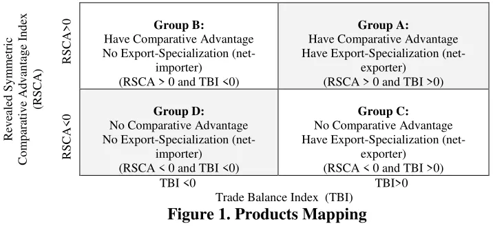
Figure 1. Products Mapping
By using the RSCA and TBI indexes, the
“
products mapping
”
is constructed. Products
(SITC)
4
can be categorized into four groups A, B, C and D as depicted in Figure 2. Group A
contains products, which have comparative advantage but no export-specialization; Group C
includes products, which have export-specialization but no comparative advantage; while, Group
D comprises products, which have neither comparative advantages nor export-specialization.
(See Appendix for the detailed calculation results)
3.3.
Econometric Model: Specialization or Despecialization?
An econometric model (3) is commonly used to examine the dynamics of comparative
advantage (Laursen, 1998; Wörz, 2005):
ij
0
,
ij
T
,
ij
RSCA
RSCA
(3)
where
RSCA
ij
,
T
and
RSCA
ij
,
0
are Revealed Symmetric Comparative Advantage of country i in
product j for the years T and 0, respectively. The coefficient
β
indicates whether existing
comparative advantage or specialization patterns have been reinforced or not during the period of
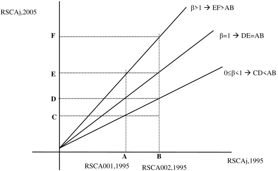
[image:12.612.175.451.444.614.2]observation.
Figure 2. Dynamic Changes in Comparative Advantages
For illustration, Figure 2 represents RSCAs for SITC 001 and SITC 002 in 1995
(horizontal axis) and 2005 (vertical axis), respectively. If
β
is not significantly different from one
(β=
1), there is no change in the overall degree of specialization. The difference between
RSCA001,1995
RSCA002,1995
A
B
C
D
E
F
0
β
<1
CD<AB
β
=1
DE=AB
β
>1
EF>AB
RSCA
001,1995
and RSCA
002,1995
(AB) equals the difference between RSCA
001,2005
and RSCA
002,2005
(DE).
β
>1 implies the increase in specialization. The difference between RSCA
001,1995
and
RSCA
002,1995
(AB) is smaller than the difference between RSCA
001,2005
and RSCA
002,2005
(EF).
Finally, 0<
β
<1 shows despecialization
–
that is, a country has gained comparative advantage in
industries where it did not specialize and has lost competitiveness in those industries where it was
initially specialized (Wörz, 2005). In the event of
β
≤
0, no reliable conclusion can be taken from
the pure statistical grounds; the specialization pattern is either random, or it has been reversed.
Since the data used in this paper is cross-section, we might have to deal with the
assumptions of the classical regression model. Conventional wisdom says that the problem of
autocorrelation is a feature of time series data and heteroscedasticity is a feature of
cross-sectional data (Gudjarati, 2000). Therefore, we can expect that heteroscedasticity might be
observed in our case. Wörz (2005) also finds that heteroscedasticity was initially a problem;
therefore, the robust standard errors computed using the
“
White/sandwich
”
5
estimator of
variance was used.
The existence of autocorrelation also might be possible. When the form of
heteroscedasticity is not known, it might not be possible to get efficient estimates of the
parameter using weighted least squares (WLS). The ordinary least squares (OLS) gives consistent
parameter estimates in the presence of heteroscedasticity but the usual OLS standard errors will
be incorrect and should not be used for the inference purposes. Therefore, this paper applies
Heteroscedasticity and Autocorrelation Consistent Covariance (HAC) when the usual OLS have
violated the homoscedasticity or no-autocorrelation assumptions
6
.
There are two possible approaches i.e. Heteroscedasticity Consistent Covariance (White)
a specific model, this paper follows some stages.
First,
the OLS is applied and then the residual
testing on heteroscedastity and autocorrelation are conducted. If the test shows that there are no
autocorrelation and heteroscedasticity simultaneously, then we apply the OLS.
Second,
if only
heteroscedasticity exists, we use the White Heteroscedasticity Consistent Covariance.
Third,
if
the autocorrelation and heteroscedasticity exist, we apply the HAC Consistent Covariances
(Newey-West).
3.4.
Correlation: convergent or divergent in the patterns of comparative advantage?
If it is believed that India’s pattern of comparative advantages follows that of China
, how
big is the time-lag? This paper applies
the Spearman’s Rank Correlation
to scrutinize the time-lag
of pattern of comparative advantage. The degree of linear association between two series of
RSCA can be compared by the Spearman’s
rank correlation coefficient, which is given as follows
(Gujarati, 2000):
1
n
n
d
6
1
2
n
1
i
2
R
b
It
,
Ct
,
s
it
a
(4)
Where:
b
It
,
Ct
,
s
a
= the Spearman’s Rank Correlation Coefficient between China’s RSCA at time t
a
(symbol: Ct
a
) and India’s RSCA at time t
b
(symbol: It
b
).
2RSCA RSCA 2 R b t , iI a t , iC
i
R
R
d
a t , iC RSCA
R
= the rank of China’s RSCA of product i at time t
a
b t , iI RSCA
R
= the rank of India’s RSCA
of product i
at time t
b
t
a
and t
b
is time (1988, 1993, 1998 or 2003)
The values of
Spearman’s rank correlation coefficients range
from
–
1 (a perfect negative
relationship) and +1 (a perfect positive relationship). The value of 0 indicates no linear
relationship. Higher
Spearman’s
rank correlation coefficient indicates stronger competition
represents that the follower catches up quickly. Negative and smaller Spe
arman’s rank
correlation
coefficient implies stronger complementarities of these two counties in supplying products to the
export market. We might
make a hypothesis that India’s
comparative advantage follows China.
4.
Results and Analysis
4.1.
“
Products mapping
”
As previously described, products (SITC) are classified into four groups i.e. A (have both
comparative advantage and specialization); B (have comparative advantage but no
export-specialization); C (have export-specialization but no comparative advantage) and D (have neither
comparative advantage nor export-specialization). Table 1 represents the percentages of the
number of products (out of 231 SITC) which lie in each group in the cases of China and India for
[image:15.612.84.529.390.535.2]the periods 1988, 1993, 1998 and 2003.
Table 1. Products Mapping: Percentage of the Number of SITC, 1988-2003
Country
1988
1993
1998
2003
China
B:
3.5%
A:
29.9%
B:
3.9%
A:
36.4%
B:
3.0%
A:
36.8%
B:
2.6%
A:
36.4%
D:
49.4%
C:
17.3%
D:
45.5%
C:
14.3%
D:
40.7%
C:
19.5%
D:
44.2%
C:
16.9%
India
B:
2.6%
A:
20.8%
B:
0.9%
A:
25.1%
B:
3.5%
A:
23.4%
B:
6.5%
A:
29.9%
D:
53.2%
C:
23.4%
D:
48.5%
C:
25.5%
D:
54.5%
C:
18.6%
D:
39.8%
C:
23.8%
Notes: A (have both comparative advantage and export-specialization); B (have comparative advantage but no export-specialization); C
(have export-specialization but no comparative advantage) and D (neither have comparative advantage nor export-specialization)
Source: International Trade Statistics Yearbook and UN-COMTRADE,
Author’s calculation.
TBI can show the
“originality”
level of a specific product. For example, if a country has
export but no import of a specific product (TBI=1), we can say that the product is originally from
the country. In contrast, if a country has import but no export of a specific product (TBI=-1), we
can say that the product is not originally from the country. Our finding shows that higher
the ‘originality’ level of products.
The higher is the level of originality, the higher will be the
level of comparative advantage
8
. In simple words, China and India have comparative advantage
on the products, which
are ‘more originally’ from
China and India. It is shown by the higher
number of products in Group A than in Group B. In contrast, the lower is the level of originality;
the lower will be the level of comparative advantage. This finding strongly supports the
Ricardian theory of comparative advantage saying that a country will have specialization in the
products with high comparative advantage.
In the case of China, the number of products in Group A increased significantly from 29.9
percent in 1988 to 36.4 percent in 2003. In contrast, the number of products in Groups A, B and
C decreased for the same periods. The biggest changes in comparative advantage and export
specialization happened in the period 1988-1993. The dramatic change in the number of products
in Group A happened from 1988 (29.9 percent) to 1993 (36.4 percent). However, it remained
relatively constant afterwards. Relatively large number of products moved from Groups C and D
to Group A rather than to Group B, indicates that import restrictions and export promotion
policies were successful in encouraging comparative advantage. It is very interesting to compare
the periods 1988-1993 and 1998-2003. What happened during 1998-2003 contradicts with what
happened during 1988-1993. Increased number of products in Group A (followed by decreased
number of products in Group B, C and D) happened during 1988-1993; while, increased number
of products in Group D (followed by decreased number of products in Groups A, B and C)
happened during 1998-2003.
In the case of India, rapid structural changes in comparative advantage and specialization
happened in 1998-2003. The number of products in Group D decreased from 54.5 percent in
1998 to 39.8 percent in 2003. It was less than that of China during the same period. In contrast,
shown that products which moved to Group A in 2003 were mainly from products in Group D in
1998. Significant increase in the number products in Group B is interesting since it shows the
increase in the
number of ‘re
-
exported’ products with high comparative advantages.
4.2. Dynamic changes in comparative advantage
China and India have long adopted trade policies for liberalization. The purpose of these
policies has been to increase the level of national welfare. Therefore, it might be theoretically
believed that China and India will try to raise their comparative advantages and to specialize in
the products with higher comparative advantages. Do China and India become more specialized
or de-specialized actually? If China and India become more specialized in specific products, the
comparative advantage of such products will become stronger than that of other products.
Table 2. Estimation Results
RSCA
Coefficients (
)
Conclusion
Coefficients (
)
Conclusion
1993 against 1988
0.742*
despecialization
0.894*
despecialization
1998 against 1993
0.845*
despecialization
0.938**
despecialization
2003 against 1998
0.875*
despecialization
0.828*
despecialization
2003 against 1988
0.485*
despecialization
0.704*
despecialization
Notes: Wald Test
9is conducted to test null hypothesis H
o
:
=1; and alternative hypothesis H
1:
1. By using 1% (*) and 5% (**) level
of significance, we do not accept hypothesis H
o.
Source: International Trade Statistics Yearbook and UN-COMTRADE,
Author’s calculation.
Table 2 represents the estimation results of equation (3) for the periods 1988-1993,
1993-1998, 1998-2003 and 1988-2003. The results confirm that China and India have generally
become less specialized for the period 1988-2003, since estimated coefficient
lies between 0
and 1 (0<
<1). The second row from the bottom of the Appendix also supports this argument by
the decrease in standard deviation of RSCA. For the period 1988-2003, China had smaller
estimated coefficient
=0.485 than that of India (0.704). It implies that change in
China’s
comparative advantages was bigger than that of India. In the case of China, the biggest change in
comparative advantage, which is shown by lowest estimated coefficient (
), happened in the
4.3. Catching-up in the patterns of comparative advantage
Different approaches of liberalization have been adopted in China and India. In the
beginning of liberalization, China was more progressive than India. As matter of fact, China has
come far ahead of India in trade and industrial development. From the third row from the bottom
of the Appendix, it is clearly shown that China has the higher average of RSCA than that of India
for 1988-2003. This sub-part describes how big is the time-lag between the two countries
’
patterns of comparative advantage. Table 3 represents the Spearman
’
s rank correlation
coefficients between the comparative advantages of China and India for the period 1988-2003.
The higher becomes the coefficient of correlation, the higher will be the linear associations of
two countries
’
comparative advantage patterns. The positive coefficient implies that India is the
[image:18.612.139.478.392.507.2]follower (if it is not called as
“
competitor
”
) of China in term of pattern of comparative advantage.
Table 3. Spearman
’
s Rank Correlation Coefficients:
China
’
s and India
’
s Comparative Advantages
India’s Comparative Advantages
1988
1993
1998
2003
Chin
a’
s
Co
mp
a
ra
tiv
e
Adv
a
nta
g
es
1988
.426*
.407*
.437*
.360*
1993
.346*
.345*
.369*
.320*
1998
.308*
.308*
.358*
.284*
2003
.316*
.278*
.311*
.221*
** Correlation is significant at the 0.01 level (2-tailed).
Source: International Trade Statistics Yearbook and UN-COMTRADE,
Author’s calculation.
To determine the time-lag, we can follow the logic shown by arrow-sign in Table 3.
First
,
comparing the coefficients
within the same column, we can find that China’s
pattern of
comparative advantages in 1988 had the highest coefficient (the arrow-sign 1). It indicates that
China’s
pattern of comparative advantages in 1988 had most similar to that of India.
Second,
across 1988, 1993, 1998 and 2003; India’s
pattern of comparative advantages in 1998 had the
highest coefficient with C
hina’s
pattern of comparative advantages in 1988 (the arrow-sign 2).
Therefore, we might say that the time-lag between India and China in term of their patterns of
(1)
(2)
comparative advantage is about 10 years (1998-1988=10 years). Interestingly, if it is the case,
then the China’s
pattern of comparative advantages in 1993 will have the higher linear
association with the India
’
s one in 2003. However, in fact it is not the case
, China’s
pattern of
comparative advantages in 1993 have higher linear association with that of India in 1998
compared with the other periods (the time-lag becomes 5 years (=1998-1993), as the arrow-sign 3
shows). Now, the time-lag becomes smaller from about 10 years to 5 years. It is very consistent
with previous explanation that the shift o
f China’s comparative advantages was quick
for the
period 1988-1993 but it was slow for the period 1993-2003. In contrast,
the shift of India’s
comparative advantages was slow for the period 1988-1998 but was fast for the period 1998-2003.
Therefore, it might be generally said that the patterns of comparative advantages of both China
and India could become similar in the near future,
ceteris paribus.
5.
Conclusions
This paper has described the trade liberalization in China and India from late 1970s up to
the present. China and India have pursued different paths of liberalization. China took the form of
‘decentralization’ of trade
, while the India
’
s core trade regime was licensing for any product. The
overall trade regime was more open in China than in India in 1980s. However, in the 1990s and
beyond both countries
’
paces of liberalization have become faster. At this stage, China has been
somewhat more open than India, though the latter has been steadily catching up the former.
Some conclusions are withdrawn.
First,
the products-mapping analysis shows that the
China’s
biggest change in comparative advantage and trade-specialization happened in
1988-1993, meanwhile the India’s one happened in 1998
-2003.
Second,
for 1988-2003, econometric
of China was bigger than that of India.
Third,
India is the follower (if it is not called
‘competitor’)
of China in term of their patterns of comparative advantages and the time-lag was about 5-10
years. As the trade patterns of the two countries become similar, the competition between them
may become the severer.
Acknowledgement
This paper is a revised and extended version of the author
’
s paper presented in the 10
th
International Conference Society for Global Business & Economic Development (SGBED)
“Creativity & Innovation: Imperative for Global Business and Development”, Kyoto, Japan
August 8-11, 2007. The author would like to thank Prof. Masumi Hakogi (Hiroshima University
of Economics), Prof. Toshiyuki Mizoguchi (Hiroshima University of Economics), Prof. Shuichi
Nakayama ((Hiroshima University of Economics), Dr. Xu Ming (China Textile University), Dr.
Katsuo C. Yamazaki (Shizuoka Sangyo University) for the valuable comments. Especially, Prof
Masumi Hakogi spent much of his time in brushing up the final version.
References
Aksoy, M.A., & Ettori, F.M., 1992.
’
Protection and industrial structure in India
’
.
Policy Research
Working Paper.
The World Bank.
Balassa, B., 1965.
‘
Trade l
iberalization and ‘
r
evealed’
comparative advantage
’
,
The Manchester
School of Economics and Social Studies
, Vol. 33, pp. 99-123.
Bloom, David, E., Caning, David, Hu, Linlin, Liu, Yuanli, Mahal, Ajay, and Yip, Winnie (2006),
Why has China’s economy taken off faster than India’s
.
Paper presented at the 2006
PAN Asia Conference, Stanford University.
Das, D.K., 2006.
China and India: A tale of two economies.
Routledge, New York.
Fan, G., and X. Zhan, 2003.’The Chinese reform agenda’. In Jost, J.T. (ed.),
Chin
a’s Role in Asia
and the World Economy.
Forum and Debt and Development (FONDAD).
Gujarati, D., 2000.
Basic Econometric
. McGraw Hill. New York.
Lardy, N., 2002.
Integrating China into the Global Economy.
Washington, D.C., Brookings
Institution Press.
Laursen, K., 1998.
‘
Revealed comparative advantage and the alternatives as measures of
international specialization
’
.
DRUID Working Paper.
No 98-30. Danish Research Unit
for Industrial Dynamics (DRUID).
Panagariya, Arvind, 2006.
‘
India and China: trade and foreign investment
’
.
Paper Presented at
‘Pan Asia 2006’ Conference
, Stanford Center for International Development,
Srinivasan, T.N., 2006.
‘
China, India and the world economy
’
.
Working Paper No. 286.
Stanford
Center for International Development. July. [online; cited 5 November 2006].
Available from URL:
http://scid.stanford.edu/pdf/SCID286.pdf
.
United Nations, 1988, 1993, 1988, 2004.
International Trade Statistics Yearbook
. The United
Nations Publsihing Section, New York.
United Nations, 2006.
United Nation Commodity Trade Statistics Database
. [online; cited 5
November 2006]. Available from
URL:http://comtrade.un.org/db/default.aspx
United Nations Conference on Trade and Development (UNCTAD), 2005.
Trade and
Development Report 2005,
New York and Geneva.
Vollrath, T.L., 1991.
‘
A theoretical evaluation of alternative trade intensity measures of revealed
comparative advantage
’
.
Weltwirtschaftliches Archiv,
127, 265-280.
Woo, W.T., 2003. ‘Challenges in macroeconomic management for China’s new leader’. In Jost,
J.T. (ed.),
China’s Role in Asia and the World Economy.
Forum and Debt and
Development (FONDAD).
World Bank, 2006.
World Development Indicators.
Washington D.C., World Bank.
World Trade Organization, 2005.
International Trade Statistic, 2005.
Geneva, World Trade
Organization.
Wörz, J., 2005. Dynamic of trade specialization in developed and less developed countries.
Appendix: Revealed Symmetric Comparative Advantage (RSCA), Trade Balance Index (TBI) and Group
No. SITC (Rev. 2) Code Descriptions
China India
RSCA TBI Group RSCA TBI Group
1988 1993 1998 2003 1988 1993 1998 2003 1988 1993 1998 2003 1988 1993 1998 2003 1988 1993 1998 2003 1988 1993 1998 2003
1 001 Live animals chiefly for food 0.52 0.35 0.19 -0.30 0.92 0.94 0.89 0.51 A A A C -0.99 -0.95 -0.96 -0.90 -0.21 0.27 0.52 0.72 D C C C
2 011 Meat and edible meat offal, fresh, chilled or frozen -0.09 -0.42 -0.21 -0.63 0.88 0.67 0.70 -0.09 C C C D -0.31 -0.30 -0.10 -0.04 1.00 1.00 1.00 1.00 C C C C
3 012 Meat and edible meat offal, in brine, dried, salted or smoked -0.11 -0.57 -0.48 -0.96 0.70 0.84 0.93 0.99 C C C C -0.86 -0.96 -0.97 -0.83 0.99 1.00 1.00 0.99 C C C C
4 014 Meat and edible meat offal, prepared, preserved, nes; fish extracts 0.61 0.46 0.18 0.26 0.97 0.99 0.99 0.98 A A A A -0.96 -0.97 -0.94 -0.92 0.96 0.92 0.99 0.75 C C C C
5 022 Milk, cream -0.82 -0.82 -0.85 -0.91 -0.57 -0.26 -0.38 -0.75 D D D D -0.97 -0.93 -0.96 -0.81 -0.97 -0.36 -0.32 -0.16 D D D D
6 023 Butter -1.00 -1.00 -0.99 -1.00 -1.00 -1.00 -0.42 -1.00 D D D D -0.91 -0.90 -0.80 -0.68 -0.92 0.66 -0.46 -0.08 D C D D
7 024 Cheese and curd -1.00 -1.00 -0.99 -1.00 -0.96 -0.94 0.28 -0.73 D D C D -0.99 -1.00 -1.00 -0.99 -0.35 -0.60 -0.46 -0.53 D D D D
8 025 Eggs, birds', and egg yolks, fresh, dried or preserved 0.53 -0.03 -0.14 -0.37 0.99 0.91 0.96 0.98 A C C C -0.85 -0.45 0.31 0.56 1.00 1.00 1.00 0.99 C C A A
9 034 Fish, fresh, chilled or frozen 0.01 0.02 0.23 0.14 0.58 0.33 0.34 0.23 A A A A -0.43 0.00 0.16 -0.16 1.00 0.97 0.83 0.93 C A A C
10 035 Fish, dried, salted or in brine; smoked fish -0.60 0.05 -0.05 -0.08 -0.15 0.28 0.45 0.62 D A C C -0.58 -0.76 -0.54 -0.33 0.99 1.00 1.00 0.97 C C C C
11 036 Crustaceans and molluscs, fresh, chilled, frozen, salted, etc 0.61 0.38 0.11 0.03 0.95 0.74 0.63 0.36 A A A A 0.78 0.79 0.81 0.75 1.00 1.00 1.00 0.99 A A A A
12 037 Crustaceans and molluscs, prepared or preserved, nes -0.43 0.26 0.52 0.53 0.95 0.97 0.99 0.98 C A A A -0.96 -0.90 -0.95 -0.06 1.00 1.00 1.00 1.00 C C C C
13 041 Wheat and meslin, unmilled -0.99 -0.96 -0.99 -0.60 -1.00 -0.98 -0.99 0.55 D D D C -0.95 -1.00 -0.99 0.57 -0.99 -1.00 -1.00 1.00 D D D A
14 042 Rice 0.58 0.40 0.55 0.07 0.41 0.76 0.77 0.67 A A A A 0.89 0.88 0.94 0.88 0.18 0.92 1.00 1.00 A A A A
15 043 Barley, unmilled -1.00 -1.00 -0.94 -0.99 -1.00 -1.00 -0.98 -0.99 D D D D -1.00 -1.00 -0.99 -1.00 0.00 0.00 1.00 0.83 D D C C
16 044 Maize, unmilled 0.43 0.71 0.26 0.50 0.94 1.00 0.89 1.00 A A A A -1.00 -0.89 -0.98 -0.11 -1.00 1.00 0.38 0.99 D C C C
17 045 Cereals, unmilled 0.40 0.18 -0.17 -0.22 1.00 1.00 0.17 0.92 A A C C -0.64 -0.13 -0.70 -0.19 -0.37 0.99 0.94 0.98 D C C C
18 046 Meal and flour of wheat and flour of meslin -0.93 -0.11 0.00 -0.36 -0.92 0.68 0.65 0.74 D C A C -1.00 -0.87 -0.82 0.67 1.00 1.00 -0.09 0.97 C C D A
19 047 Other cereal meals and flour -0.23 -0.41 -0.57 -0.58 0.94 0.76 -0.02 0.69 C C D C -0.96 -0.49 -0.34 0.10 -0.95 0.99 -0.78 0.95 D C D A
20 048 Cereal, flour or starch preparations of fruits or vegetable -0.44 -0.57 -0.77 -0.77 0.68 0.58 0.68 0.18 C C C C -0.49 -0.61 -0.63 -0.55 -0.68 -0.03 0.49 0.57 D D C C
21 054 Vegetables, fresh or simply preserve; roots and tubers, nes 0.43 0.37 0.20 0.01 0.94 0.95 0.89 0.76 A A A A -0.04 -0.09 -0.03 0.06 -0.63 -0.33 -0.15 -0.29 D D D B
22 056 Vegetables, roots and tubers, prepared or preserved, nes 0.77 0.71 0.66 0.57 1.00 0.99 0.97 0.98 A A A A -0.31 -0.13 0.01 0.11 1.00 1.00 0.87 0.86 C C A A
23 057 Fruit and nuts, fresh, dried -0.09 -0.26 -0.47 -0.57 0.70 0.76 0.21 0.12 C C C C 0.42 0.48 0.43 0.28 0.47 0.28 0.08 0.07 A A A A
24 058 Fruit, preserved, and fruits preparations 0.11 0.02 0.10 0.15 0.94 0.82 0.94 0.83 A A A A -0.20 -0.29 -0.22 -0.60 1.00 1.00 0.90 0.54 C C C C
25 061 Sugar and honey -0.32 0.40 -0.37 -0.66 -0.79 0.71 0.16 -0.08 D A C D -0.79 -0.13 -0.76 0.45 0.34 0.81 -0.92 0.82 C C D A
26 062 Sugar confectionery and preparations, non-chocolate -0.57 -0.17 -0.48 -0.42 0.12 0.47 0.55 0.73 C C C C -0.84 -0.90 -0.85 -0.58 1.00 0.89 -0.03 0.54 C C D C
27 071 Coffee and coffee substitutes -0.98 -0.97 -0.90 -0.88 -0.72 -0.15 0.43 0.37 D D C C 0.50 0.55 0.61 0.48 1.00 1.00 0.98 0.95 A A A A
28 072 Cocoa -0.48 -0.62 -0.75 -0.91 -0.20 0.02 -0.16 -0.40 D C D D -0.91 -0.98 -1.00 -0.99 0.99 -0.31 -0.99 -0.93 C D D D
29 073 Chocolate & other food preparations containing cocoa, nes -0.82 -0.84 -0.94 -0.91 0.73 0.27 -0.27 -0.26 C C D D -0.96 -0.97 -0.91 -0.91 1.00 0.90 0.08 -0.22 C C C D
30 074 Tea and mate 0.87 0.76 0.61 0.36 0.89 0.98 0.99 0.98 A A A A 0.96 0.93 0.94 0.87 1.00 0.99 0.94 0.92 A A A A
31 075 Spices 0.46 0.53 0.27 0.20 0.69 0.86 0.92 0.93 A A A A 0.91 0.90 0.91 0.83 0.69 0.79 0.66 0.42 A A A A
32 081 Feeding stuff for animals (not including unmilled cereals) 0.56 0.00 -0.55 -0.58 0.40 0.19 -0.73 -0.21 A C D D 0.57 0.74 0.57 0.54 0.98 0.94 0.88 0.81 A A A A
33 091 Margarine and shortening -0.98 -0.95 -0.55 -0.81 -0.98 -0.86 0.28 -0.14 D D C D -0.56 -0.42 -0.59 -0.65 0.98 0.97 -0.88 0.55 C C D C
Appendix:
Continued……
No. SITC (Rev. 2) Code Descriptions
China India
RSCA TBI Group RSCA TBI Group
1988 1993 1998 2003 1988 1993 1998 2003 1988 1993 1998 2003 1988 1993 1998 2003 1988 1993 1998 2003 1988 1993 1998 2003
35 111 Non-alcoholic beverages, nes 0.53 0.32 0.33 -0.22 0.68 0.68 0.98 0.97 A A A C -0.97 -0.95 -0.98 -0.94 1.00 1.00 -0.32 -0.62 C C D D
36 112 Alcoholic beverages -0.69 -0.65 -0.82 -0.85 0.40 0.74 0.19 0.07 C C C C -0.96 -0.83 -0.87 -0.88 -0.50 0.59 0.16 0.19 D C C C
37 121 Tobacco, unmanufactured; tobacco refuse -0.28 0.01 -0.11 -0.19 -0.35 0.46 0.68 -0.07 D A C D 0.50 0.57 0.55 0.57 1.00 0.99 0.93 0.96 A A A A
38 122 Tobacco, manufactured -0.50 0.14 -0.23 -0.59 -0.63 0.54 0.70 0.70 D A C C -0.41 -0.52 -0.43 -0.38 0.87 0.92 0.90 0.77 C C C C
39 211 Hides and skins, excluding furs, raw 0.07 -0.66 -0.83 -0.97 0.44 -0.65 -0.91 -0.99 A D D D -1.00 -0.94 -0.99 -0.87 -1.00 -0.94 -1.00 -0.88 D D D D
40 212 Furskins, raw 0.13 -0.33 -0.68 -0.92 0.41 -0.73 -0.68 -0.90 A D D D -1.00 -1.00 -1.00 -0.99 -1.00 -1.00 -1.00 0.13 D D D C
41 222 Seeds and oleaginous fruit, whole broken, for 'soft' fixed oil 0.57 0.26 -0.29 -0.40 0.89 0.87 -0.64 -0.82 A A D D -0.40 0.09 0.07 0.33 0.97 1.00 0.99 0.99 C A A A
42 223 Seeds and oleaginous fruit, whole broken, for other fixed oils 0.66 0.33 -0.41 -0.16 0.99 0.92 0.46 0.75 A A C C 0.57 0.57 0.53 0.47 0.29 0.56 0.61 0.28 A A A A
43 232 Natural rubber, latex; rubber and gums -1.00 -0.90 -0.84 -0.99 -1.00 -0.95 -0.92 -1.00 D D D D -0.98 -0.99 -0.91 0.01 -0.99 -0.98 -0.89 0.08 D D D A
44 233 Synthetic rubber, latex, etc; waste, scrap of unhardened rubber -0.84 -0.72 -0.76 -0.67 -0.80 -0.84 -0.89 -0.86 D D D D -0.91 -0.79 -0.73 -0.60 -0.96 -0.93 -0.91 -0.87 D D D D
45 244 Cork, natural, raw & waste -0.99 -0.84 -0.97 -0.84 -0.99 -0.86 -0.95 -0.67 D D D D -1.00 -0.92 -0.96 -0.82 -1.00 -0.96 -0.97 -0.68 D D D D
46 245 Fuel wood and wood charcoal -0.90 0.07 0.52 0.38 -0.44 0.86 0.94 0.93 D A A A -0.98 -0.71 -0.74 -0.25 -0.89 1.00 0.68 0.73 D C C C
47 246 Pulpwood (including chips and wood waste) -0.70 0.15 0.34 -0.13 -0.29 0.86 0.91 0.49 D A A C -1.00 -1.00 -1.00 -1.00 0.00 -1.00 -1.00 -0.90 D D D D
48 247 Other wood in the rough or roughly squared -0.32 -0.55 -0.91 -0.99 -0.88 -0.73 -0.96 -1.00 D D D D -0.94 -1.00 -0.97 -0.92 -0.99 -1.00 -1.00 -0.99 D D D D
49 248 Wood, simply worked and railway sleepers of wood -0.83 -0.60 -0.69 -0.61 -0.39 -0.08 -0.40 -0.48 D D D D -0.99 -1.00 -0.99 -0.97 -0.97 -0.94 -0.87 -0.56 D D D D
50 251 Pulp and waste paper -0.97 -0.98 -0.97 -0.97 -0.98 -0.97 -0.98 -0.99 D D D D -1.00 -0.99 -0.98 -0.99 -1.00 -1.00 -0.99 -1.00 D D D D
51 261 Silk 0.96 0.95 0.96 0.96 0.96 0.99 0.91 0.92 A A A A -0.11 -0.52 0.65 0.04 -0.83 -0.98 -0.69 -0.96 D D B B
52 263 Cotton 0.77 0.10 -0.72 -0.61 0.85 0.80 -0.73 -0.80 A A D D -0.37 0.64 -0.13 0.46 -0.64 0.94 -0.29 -0.24 D A D B
53 265 Vegetable textile fibers, excluding cotton, jute, and waste 0.74 0.47 -0.11 -0.69 0.96 0.32 -0.56 -0.92 A A D D -0.97 -0.79 -0.18 0.07 -0.98 -0.95 -0.35 0.01 D D D A
54 266 Synthetic fibers suitable for spinning -0.92 -0.87 -0.53 -0.29 -0.99 -0.98 -0.91 -0.77 D D D D 0.09 -0.40 -0.23 0.10 0.08 -0.56 -0.52 0.11 A D D A
55 267 Other man-made fibres suitable for spinning, and waste -0.69 -0.90 -0.85 -0.93 -0.94 -0.89 -0.96 -0.97 D D D D -0.84 -0.56 -0.64 -0.11 -0.75 -0.45 -0.69 -0.15 D D D D
56 268 Wool and other animal hair (including wool tops) 0.56 0.47 0.27 0.28 -0.33 -0.30 -0.39 -0.41 B B B B -0.60 -0.95 -0.72 -0.70 -0.85 -0.99 -0.95 -0.95 D D D D
57 269 Old clothing and other old textile articles, rags -0.47 -0.71 -0.77 -0.93 0.74 0.21 0.44 -0.15 C C C D -0.84 -0.92 -0.81 -0.13 -0.98 -0.98 -0.93 -0.77 D D D D
58 271 Fertilizers, crude -0.75 -0.21 0.25 0.27 -0.48 0.24 0.95 0.93 D C A A -1.00 -0.97 -0.93 -0.89 -1.00 -1.00 -1.00 -0.99 D D D D
59 273 Stone, sand and gravel 0.11 0.16 -0.10 -0.24 0.98 0.79 0.01 -0.54 A A C D 0.79 0.78 0.72 0.80 0.87 0.89 0.60 0.73 A A A A
60 274 Sulfur and unroasted iron pyrites -0.46 -0.91 -0.82 -0.84 0.58 -0.40 -0.91 -0.98 C D D D -0.99 -0.97 -0.84 -0.76 -1.00 -1.00 -0.99 -0.98 D D D D
61 277 Natural abrasives, nes 0.18 -0.23 -0.30 -0.57 0.48 0.18 0.21 -0.23 A C C D 0.47 0.27 0.38 0.44 0.74 0.19 0.38 0.23 A A A A
62 278 Other crude minerals 0.61 0.50 0.54 0.32 0.95 0.88 0.74 0.52 A A A A 0.28 -0.10 -0.02 0.14 -0.28 -0.39 -0.39 -0.15 B D D B
63 281 Iron ore and concentrates -1.00 -1.00 -1.00 -1.00 -1.00 -1.00 -1.00 -1.00 D D D D 0.83 0.79 0.73 0.85 0.99 0.94 0.97 0.87 A A A A
64 282 Waste and scraps metal or iron or steel -0.05 -0.95 -0.95 -1.00 0.52 -0.98 -0.94 -1.00 C D D D -0.81 -0.97 -0.95 -0.94 -0.99 -0.99 -0.99 -0.99 D D D D
65 287 Ores and concentrates of base metals, nes 0.16 -0.65 -0.77 -0.71 0.19 -0.72 -0.87 -0.88 A D D D 0.46 0.26 -0.03 0.21 0.47 0.56 -0.30 -0.15 A A D B
66 288 Non-ferrous base metal waste and scrap, nes -0.81 -0.73 -0.84 -0.88 0.14 -0.83 -0.90 -0.96 C D D D -0.99 -0.99 -0.91 -0.21 -1.00 -1.00 -0.98 -0.67 D D D D
67 289 Ores & concentrates of precious metal, waste, scrap -0.98 0.88 -0.98 -0.89 0.46 1.00 -0.74 0.48 C A D C -1.00 -1.00 -1.00 -0.68 -1.00 -0.97 -0.82 0.08 D D D C
68 291 Crude animal materials, nes 0.86 0.71 0.73 0.56 0.85 0.82 0.73 0.54 A A A A 0.56 0.40 0.28 0.04 0.89 0.84 0.59 0.55 A A A A
Appendix:
Continued……
No. SITC (Rev. 2) Code Descriptions
China India
RSCA TBI Group RSCA TBI Group
1988 1993 1998 2003 1988 1993 1998 2003 1988 1993 1998 2003 1988 1993 1998 2003 1988 1993 1998 2003 1988 1993 1998 2003
70 322 Coal, lignite and peat 0.33 0.18 0.24 0.37 0.79 0.89 0.88 0.76 A A A A -0.81 -0.71 -0.57 -0.51 -0.94 -0.91 -0.92 -0.89 D D D D
71 323 Briquettes, coke and semi-coke; lignite or peat; retort carbon 0.45 0.65 0.88 0.86 0.99 0.99 1.00 1.00 A A A A -0.89 -0.94 -0.98 -0.87 -0.92 -0.96 -1.00 -0.99 D D D D
72 333 Crude petroleum and oils obtained from bituminous minerals 0.10 -0.31 -0.61 -0.87 0.93 0.02 -0.37 -0.85 A C D D -1.00 -1.00 -1.00 -0.99 -1.00 -1.00 -1.00 -1.00 D D D D
73 334 Petroleum products, refined -0.25 -0.56 -0.63 -0.51 0.16 -0.65 -0.54 -0.24 C D D D 0.02 -0.15 -0.73 0.38 -0.51 -0.71 -0.93 0.32 B D D A
74 335 Residual petroleum products, nes and related materials 0.25 0.19 0.24 -0.21 0.45 0.47 0.33 -0.40 A A A D -0.98 -0.94 -0.60 0.17 -0.98 -0.96 -0.94 -0.13 D D D B
75 341 Gas, natural and manufactured -0.99 -0.99 -0.81 -0.95 -0.46 -0.97 -0.61 -0.84 D D D D -1.00 -0.47 -0.96 -0.96 -0.72 0.15 -0.96 -0.93 D C D D
76 411 Animal oils and fats -0.99 -0.96 -0.91 0.82 -0.99 -0.97 -0.93 0.66 D D D A -0.96 -0.96 -0.92 -0.79 -0.22 -0.58 -0.58 -0.20 D D D D
77 423 Fixed vegetable oil, soft, crude refined or purified -0.70 -0.26 -0.37 -0.88 -0.69 -0.13 -0.55 -0.92 D D D D -1.00 -0.96 -0.98 -0.56 -1.00 -0.94 -1.00 -0.91 D D D D
78 424 Other fixed vegetable oils, fluid or solid, crude, refined 0.00 -0.07 -0.63 -0.90 -0.61 -0.52 -0.81 -0.95 B D D D -0.38 0.50 0.44 0.13 -0.95 0.43 -0.77 -0.87 D A B B
79 431 Animal and vegetable oils and fats, processed, and waxes -0.90 -0.79 -0.64 -0.88 -0.31 -0.05 0.19 -0.73 D D C D -0.80 -0.20 0.06 0.30 -0.89 -0.61 -0.72 -0.29 D D B B
80 511 Hydrocarbons, nes and derivatives -0.80 -0.66 -0.58 -0.56 -0.84 -0.67 -0.65 -0.78 D D D D -0.70 -0.35 -0.11 0.30 -0.83 -0.80 -0.71 -0.26 D D D B
81 512 Alcohols, phenols etc, and their derivatives -0.19 -0.20 -0.37 -0.48 -0.42 -0.31 -0.52 -0.79 D D D D -0.44 -0.25 0.05 -0.04 -0.82 -0.38 -0.29 -0.47 D D B D
82 513 Carboxylic acids and their derivatives -0.09 -0.10 -0.03 -0.17 -0.45 -0.18 -0.26 -0.64 D D D D -0.61 -0.28 -0.13 0.05 -0.66 -0.43 -0.43 -0.22 D D D B
83 514 Nitrogen-function compounds -0.52 -0.43 -0.34 -0.34 -0.68 -0.14 0.02 -0.10 D D C D 0.19 0.00 -0.05 -0.13 0.07 0.13 -0.06 -0.19 A A D D
84 515 Organo-inorganic and heterocyclic compounds -0.08 -0.09 -0.11 -0.34 -0.26 0.11 0.24 0.07 D C C C -0.59 -0.29 -0.22 -0.32 -0.78 -0.32 -0.12 -0.04 D D D D
85 516 Other organic chemicals -0.38 -0.22 0.07 -0.16 -0.24 0.19 0.15 -0.15 D C A D -0.33 0.19 0.70 0.78 -0.82 -0.39 0.20 0.32 D B A A
86 522 Inorganic chemical elements, oxides, and halogen salts 0.29 0.32 0.37 0.24 0.38 0.66 0.57 0.38 A A A A -0.66 -0.49 -0.23 -0.15 -0.96 -0.90 -0.90 -0.81 D D D D
87 523 Other inorganic chemicals; compounds of precious metals 0.35 0.33 0.44 0.37 0.00 0.49 0.58 0.53 B A A A -0.18 -0.13 -0.11 0.07 0.05 0.08 -0.26 -0.10 C C D B
88 524 Radioactive and associated materials 0.05 0.06 0.24 -0.26 0.96 0.94 0.80 0.44 A A A C -0.97 -0.99 -0.96 -0.95 0.93 -0.15 -0.17 -0.10 C D D D
89 531 Synthetic dye, natural indigo, lakes 0.02 0.07 0.33 0.24 0.00 0.11 0.44 0.31 A A A A 0.57 0.70 0.71 0.74 0.84 0.85 0.77 0.75 A A A A
90 532 Dyeing and tanning extracts; synthetic tanning materials -0.70 -0.23 -0.53 -0.14 -0.06 -0.10 -0.58 -0.39 D D D D -0.22 -0.07 0.26 0.42 -0.77 -0.74 -0.59 -0.34 D D B B
91 533 Pigments, paints, varnishes and related materials -0.20 -0.49 -0.43 -0.56 -0.03 -0.53 -0.44 -0.57 D D D D 0.01 -0.70 -0.74 -0.48 0.14 -0.42 -0.65 -0.38 A D D D
92 541 Medicinal and pharmaceutical products -0.07 -0.19 -0.33 -0.63 0.10 0.37 0.52 0.25 C C C C 0.22 0.45 0.23 0.08 0.22 0.53 0.42 0.52 A A A A
93 551 Essential oils, perfume and flavor materials 0.30 -0.08 -0.42 -0.73 0.63 0.64 0.37 -0.11 A C C D 0.23 0.09 0.14 0.05 0.27 0.39 0.39 0.39 A A A A
94 553 Perfumery, cosmetics, toilet preparation, etc -0.47 -0.47 -0.60 -0.54 0.61 0.74 0.68 0.67 C C C C 0.29 -0.09 -0.17 -0.21 0.89 0.92 0.68 0.63 A C C C
95 554 Soap, cleansing and polishing preparations -0.44 -0.51 -0.56 -0.70 -0.15 -0.29 -0.20 -0.34 D D D D -0.14 0.00 -0.55 -0.50 0.15 0.42 -0.37 -0.13 C A D D
96 562 Fertilizers, manufactured -0.83 -0.74 -0.57 -0.08 -0.98 -0.94 -0.89 -0.38 D D D D -0.99 -0.89 -0.87 -0.90 -1.00 -0.99 -0.98 -0.97 D D D D
97 572 Explosives and pyrotechnic products 0.91 0.67 0.76 0.64 1.00 0.98 0.99 0.97 A A A A -0.52 -0.32 -0.20 -0.31 -0.03 0.80 0.75 0.44 D C C C
98 582 Condensation, polycondensation and polyaddition products -0.90 -0.83 -0.56 -0.48 -0.93 -0.90 -0.73 -0.71 D D D D -0.83 -0.57 -0.25 -0.05 -0.71 -0.35 -0.18 -0.08 D D D D
99 583 Polymerization and copolymerization products -0.78 -0.74 -0.64 -0.77 -0.95 -0.90 -0.86 -0.88 D D D D -0.90 -0.82 -0.71 -0.14 -0.96 -0.85 -0.73 0.06 D D D C
100 584 Regenerated cellulose, derivatives or cellulose, vulcanized fibre -0.74 -0.71 -0.74 -0.63 -0.60 -0.79 -0.80 -0.49 D D D D -0.74 -0.73 -0.62 -0.36 -0.47 -0.61 -0.71 -0.43 D D D D
101 585 Other artificial resins and plastic materials -0.18 0.49 0.46 0.44 0.62 0.72 0.76 0.74 C A A A -0.98 -0.40 -0.33 -0.41 -0.89 0.35 -0.14 -0.28 D C D D
102 591 Pesticides, disinfectants -0.40 -0.37 -0.10 -0.02 0.99 -0.16 0.27 0.69 C D C C 0.14 0.12 0.50 0.56 0.37 0.57 0.68 0.55 A A A A
103 592 Starches, insulin and wheat gluten, albuminoidal substances; glues -0.54 -0.61 -0.51 -0.41 -0.17 -0.63 -0.53 -0.40 D D D D -0.92 -0.79 -0.42 -0.26 -0.66 -0.20 0.09 0.13 D D C C