Munich Personal RePEc Archive
Decimalization, Realized Volatility, and
Market Microstructure Noise
Vuorenmaa, Tommi A.
University of Helsinki
April 2008
Online at
https://mpra.ub.uni-muenchen.de/8692/
öMmföäflsäafaäsflassflassflas ffffffffffffffffffffffffffffffffffff
Discussion Papers
Decimalization, Realized Volatility, and Market
Microstructure Noise
Tommi A. Vuorenmaa
University of Helsinki and HECER
Discussion Paper No. 217 May 2008
ISSN 1795-0562
HECER – Helsinki Center of Economic Research, P.O. Box 17 (Arkadiankatu 7), FI-00014 University of Helsinki, FINLAND, Tel +358-9-191-28780, Fax +358-9-191-28781,
HECER
Discussion Paper No. 217
Decimalization, Realized Volatility, and Market
Microstructure Noise*
Abstract
This paper studies empirically the effect of decimalization on volatility and market microstructure noise. We apply several non-parametric estimators in order to accurately measure volatility and market microstructure noise variance before and after the final stage of decimalization which, on the NYSE, took place in January, 2001. We find that decimalization decreased observed volatility by decreasing noise variance and, consequently, increased the significance of the true signal especially in the trade price data for the high-activity stocks. In general, however, most of the found increase in the signal-to-noise ratio is explainable by confounding and random effects. We also find that although allowing for dependent noise can matter pointwisely, it does not appear to be critical in our case where the estimates are averaged over time and across stocks. For that same reason rare random jumps are not critical either. It is more important to choose a proper data type and prefilter the data carefully.
JEL Classification: C14, C19.
Keywords: Decimalization; Market microstructure noise; Realized volatility; Realized variance; Tick size; Ultra-high-frequency data.
Tommi A. Vuorenmaa
Department of Economics University of Helsinki
P.O. Box 17 (Arkadiankatu 7) FI-00014 University of Helsinki FINLAND
e-mail:[email protected]
Introduction
The New York Stock Exchange (NYSE) completed its long anticipated change from
fractional pricing to decimal pricing on January 29, 2001. This process is known as
"decimalization." It is accompanied by a reduction in the minimum price variation called
the tick size which in this case is from a sixteenth of a dollar to one cent. A reduction
in tick size can have significant effects on other variables because it removes constraints on pricing and makes the cost of obtaining price priority smaller. This in turn may
change the strategic behavior of the players in the market. The effect of decimalization
on the quoted bid-ask spread, trading volume, and alike are well documented. The
effects on more elaborate concepts are not as clear, however. Although volatility is
almost unanimously reported to decrease [see, e.g., Ronen and Weaver (2001)], most of
the empirical studies use unprecise estimation methods and sparsely sampled data that
weaken the results. And with only very few exceptions [He and Wu (2005)] do these
studies decompose volatility in any way.
In theory, price discreteness forces the observed price to deviate from the "true"
price [see, e.g., Gottlieb and Kalay (1985), Cho and Frees (1988), and Easley and
O’Hara (1992)]. As a consequence, the observed volatility is upward biased relatively
to the true volatility by amount that depends on the tick size [see Harris (1990a)] and
the sampling frequency [see, e.g., Gottlieb and Kalay (1985)]. Because decimalization
alleviates rounding errors, the difference between the true and the observed price should
narrow. This should damp the observed volatility but leave the true volatility intact.
Hansen and Lunde (2006)find some evidence in this direction.
In this paper, we let the observed volatility to consist of two additive components:
the true volatility and the market microstructure noise variance. This decomposition
allows us to estimate them separately. If noise would not be separated out, the estimated
volatility would depend on the sampling frequency through the noise term and cause
this, we use elaborate econometric estimation methods that allow us to extract useful
information from ultra-high-frequency (UHF) data. We take advantage of the fact
that the NYSE decimalization was carried out in a manner that resembles a controlled
natural experiment. We also use mixed-effect panel regressions to ensure that the found
effects are not caused by confounding factors or randomness.
A key point is tofirst estimate the true volatility accurately. As noted for example by Cho and Frees (1988), the sample standard deviation underestimates the true
stan-dard deviation even in the absence of noise. We use several non-parametric estimators
that have desirable statistical properties and are yet flexible and simple to calculate. In particular, if the market microstructure noise is IID, then the two-scale realized
volatility (TSRV) estimator [Zhang, Mykland, and Aït-Sahalia (2005)] is consistent
and unbiased. Similarly, the re-scaled realized volatility estimator provides consistent
noise variance estimates. Both variance measures carry economically significant infor-mation [Bandi and Russell (2006)]. Their ratio, "signal-to-noise," allows us to evaluate
changes in the composition of volatility.
We also let the market microstructure noise to be serially correlated. The generalized
TSRV [Aït-Sahalia, Mykland, and Zhang (2006)] and the multi-scale realized volatility
[Zhang (2005)] estimators are then still consistent and unbiased. The latter estimator,
in particular, is able to account for time varying noise properties. Such flexibility is welcome because the properties of noise have been shown to vary over time and data
type [see Hansen and Lunde (2006)]. We demonstrate how the volatility estimators
cope with the change in tick size. This also enables us to study if decimalization affects
the trade price and midquote estimates differently.
Finally, because jumps can have a deteriorating effect on the estimates of volatility
and market microstructure noise variance [see Fan and Wang (2006)], we investigate
the presence of jumps by a simple and direct test recently proposed by Aït-Sahalia and
Jacod (2006). We find that jumps do exist, as expected, and that their impact may be different in event and calendar time. We then remove the jumps using different
random events, and because in our analysis we take averages over time and across
stocks, we do not expect to see qualitatively significant changes in our results.
The empirical results of this paper show how a tick size reduction affects volatility
and market microstructure noise. As argued by Harris (1990a), price discreteness can
produce significant biases especially when small variance components are being iden-tified from UHF data. This is relevant for example to risk management and options pricing [see Figlewski (1997)]. Our results should also be of interest to stock exchanges
and institutions that work on to improve the efficiency of the markets. International
volatility spillovers combined with the recent collusions between major stock exchanges
highlight the need for rules that help to weigh down excess volatility (consider the
NYSE—Euronext and Nasdaq—OMX mergers). In the future it may for example be
that a tick size different from one cent is found optimal or that more advanced trading
mechanisms are introduced in order to reduce market microstructure noise. After all,
stock prices should ideally reflect all known information and not noise [see Black (1986) and Amihud and Mendelson (1987)].
The structure of this paper is as follows. In Section 1, we review the related
deci-malization literature. In Section 2, we describe the estimators we use in the empirical
study. The data are described in Section 3. In Section 4, we report the empirical
re-sults. We conclude in Section 5. Appendix includes additional tables with volatility
estimates and also illustrates the idea of subsampling and averaging that the estimators
are based on.
1
Review of decimalization e
ff
ects
This section gives a brief review of the relevant decimalization literature. [A more
general survey can be found for example in Harris (1997, 1999) and NYSE (2001).]
Notice that different methods and data sets make comparisons of many decimalization
eights to sixteenths does not necessarily have the same effect as a tick size decrease
from sixteenths to cents.
The most direct evidence concerns the (bid-ask) spread. Both absolute and relative
spreads have been found to decrease. As predicted for example by the Harris (1994)
model, Ahn, Cao, and Choe (1996) and Ronen and Weaver (2001) find that the tick size decrease from eights to sixteenths reduced the quoted and effective spreads on
the American Stock Exchange (AMEX). Similar evidence is reported for the change to
five cents on the Toronto Stock Exchange (TSE) [e.g., Bacidore (1997)], from eights to sixteenths on the NYSE [Ricker (1998), Bollen and Whaley (1998), and Goldstein
and Kavajecz (2000)], and from sixteenths to cents on the NYSE and the Nasdaq
[Bessembinder (2003)]. Goldstein and Kavajecz (2000) and Bessembinder (2003) note
that the spread decrease is largest for the most active stocks.
The Harris (1994) model also predicts a decrease in quoted depth and an increase
in trading volume. Ahn, Cao, and Choe (1996) and Ronen and Weaver (2001) however
find no significant changes in quoted depth or trading activity on the AMEX. On the other hand, Bacidore (1997) and Porter and Weaver (1997)find depth to decrease but trading volume to remain constant on the TSE. Ricker (1998), Bollen and Whaley
(1998), Goldstein and Kavajecz (2000), and Bacidore, Battalio, and Jennings (2001)
report decreases in quoted depth on the NYSE. van Ness, van Ness, and Pruitt (1999)
report increases in the number of trades and volume. Chakravarty, van Ness, and van
Ness (2005) report an increase in the volume of small sized trades.
Ricker (1998), Bollen and Whaley (1998), and Bacidore, Battalio, and Jennings
(2001)find that decimalization improved liquidity on the NYSE. Bessembinder (2003) does not find evidence of liquidity problems on the Nasdaq either. It is indisputable, however, that displayed liquidity is decreased because of more order cancellations and
smaller limit order sizes. NYSE (2001), among others, concludes that market
trans-parency diminished. Jones and Lipson (2001) point out that the spread is no longer a
sufficient statistic of market quality for large investors. They report increased average
from eights to sixteenths. Similar evidence is presented by Goldstein and Kavajecz
(2000). In contrast, Chakravarty, Panchapagesan, and Wood (2005) do not find evi-dence of liquidity problems due to change to cents using NYSE Plexus data [in line
with Bacidore, Battalio, and Jennings (2003)]. They suggest that large investors may
have started using more cautious execution strategies.
Because liquidity does not appear to be adversely affected (at least not too much),
decimalization is unlikely to increase volatility. Notice, however, that the great recent
increase of algorithmic trading [see Economist (2007b)] — partly fueled by the diminished
market transparency and the higher market making costs due to decimalization itself —
may have actually made the markets more sensitive to bad news. Trading algorithms
can trigger sell-offs which in turn may cause losses of liquidity as happened for example
in October 1987 when the widely adopted "portfolio insurance" strategies fully kicked
in. More recent evidence is from February 2007 when automated trading led to severe
order-routing problems on the NYSE [see Economist (2007a)]. These instances are of
course expected to be rare by standard measures.1 In "normal periods" decimalization
is likely to decrease volatility due to the smaller impact of price discreteness.2 Indeed,
Ronen and Weaver (2001) and Bessembinder (2003) report volatility reductions on the
AMEX, the NYSE, and the Nasdaq. Both studies proxy volatility by standard deviation
or variance of midquote returns (the former also uses daily closing midquotes).3 They
do not find exogenous market trends to be responsible for the decrease. Chakravarty, Wood, and van Ness (2004) report similar findings for portfolio volatility constructed from one minute intraday returns that are volume weighted.
It remains to identify what factors actually reduced volatility. A volatility reduction
may be due to many different components such as the bid-ask bounce, price
adjust-1There is also evidence that algorithmic trading improves liquidity instead of decreasing it [see
Hendershott, Jones, and Menkveld (2008)], that is, at least during "troubless" normal times.
2Ikenberry and Weston (2003) and Chung, van Ness, and van Ness (2004) howeverfind significant
clustering to five and ten cents after decimalization so that the impact may not be full. Clustering is not that surprising, though, because it simplifies price negotiation, among other things [see, e.g., Harris (1991)].
3As noted for example by Cho and Frees (1988), Jensen’s inequality can be used to show that the
ments to large trades, price discreteness, and so on. Market microstructure noise can
be driven by information asymmetries between the traders and the market maker. Not
surprisingly, identification of the factors is hard in practice. Conflicting evidence of for example whether adverse selection was increased or decreased exists [see Zhao and
Chung (2006), Chakravarty, van Ness, and van Ness (2005), and Bacidore (1997)].
Per-haps most relevantly to us, He and Wu (2005) decompose the variance of price changes
into public news, price discreteness, and bid-ask spreads using the method of Madhavan,
Richardson, and Roomans (1997). Theyfind a significant variance decline due to price discreteness and spreads. Gibson, Singh, and Yerramilli (2003) furthermore find that the spread reduction on the NYSE is due to a decrease in the order-processing
compo-nent (and that inventory and adverse selection compocompo-nents remain significant). Engle and Sun (2005) find that in the decimalized NYSE as much as 86% of the variance of market microstructure noise in transactions can be due to variation in the informational
component (the rest due to the non-informational component). In this paper, however,
we treat market microstructure noise as a one unit and do not attempt to separate out
its components.
2
Estimators
The framework in which we operate is standard. It can be viewed as a reduced form of
structural market microstructure models such as the model of Madhavan, Richardson,
and Roomans (1997) [see the discussion in Hasbrouck (1996)]. We now shortly review
it.
Let the observed price, Y, consist of the latent true price X and noise :
Yti =Xti + ti. (1)
effects, and so on. In the IID case the first-order autocovariance of the (observed) returns can be shown to be−E 2 (and zero afterwards) [see, e.g., Aït-Sahalia, Mykland,
and Zhang (2006)]. Because trades and quotes tend to cluster over time, this framework
has been extended to include serially dependent noise. Hansen and Lunde (2006) argue
it to be particularly relevant with very frequent sampling in a decimalized market
like ours. We take dependent noise into account by using proper estimation methods
(described below).
In Eq. (1), the true (generally unobserved) (log)price X is standardly assumed to follow an Itô process,
dXt=μtdt+σtdBt,
withσtpossibly stochastic andBtthe standard Brownian motion.4 Changes in the true price are believed to be information driven and they are permanent. This is in line with
the view that the true price process should be positively correlated [see, e.g., Amihud
and Mendelson (1987)]. Standardly, the true price is also assumed to be independent of
the noise process. Although Hansen and Lunde (2006) argue that in practice negative
dependence exists especially in the midquote data due to severe asymmetric information
effects [see, e.g., Glosten and Milgrom (1985) and Madhavan, Richardson, and Roomans
(1997)], in this paper we maintain the assumption of independence [for more discussion,
see Aït-Sahalia, Mykland, and Zhang (2005b)].
If volatility is stochastic, it is important in many financial applications (e.g., in option pricing) to estimate the so-called integrated volatility (IV),
hX, XiT = Z T
0
σ2tdt,
as accurately as possible. Without any noise arising from market microstructure,
real-4Itô processes include for example the Ornstein—Uhlenbeck process as a special case. The true price
ized volatility (RV), also known as quadratic variation (in the theoretical limit),
[Y, Y](Tall)= n−1
X
i=0
¡
Yti+1−Yti
¢2
over the observed prices at times0 = t0 < t1 <· · ·< tn=T,provides a precise estimate of IV as∆t→0(sampling higher).5 In the presence of noise it does not, however. With
IID noise, RV provides a consistent estimate of the noise variance instead [see Zhang,
Mykland, Aït-Sahalia (2005) and Bandi and Russell (2003)]:
1
2n[Y, Y]
(all)
T =dE 2. (2)
We call this noise variance estimator the re-scaled realized volatility (RSRV). Because
of its upward biasedness [see Oomen (2005b) and Hansen and Lunde (2006)], we also
present a popular unbiased noise variance estimator later on (based on the
aforemen-tioned fact that thefirst-lag autocovariance term of returns equals −E 2).6
Several more precise estimators for IV have been proposed [see, e.g., Zhou (1996)].
Although most of them provide an unbiased estimate of IV, only few of them are
consistent. In this paper we use three estimators that are not only unbiased but also
consistent. These estimators all are based on the idea of subsampling and averaging,
and although they start to be well known by now, we next describe them in some detail.
The reader mayfind the details useful in the empirical section where we carry out some qualitative robustness checks.
The TSRV estimator of Zhang, Mykland, and Aït-Sahalia (2005) is defined as
\
hX, Xi(Ttsrv) = [Y, Y](TK)−n
n[Y, Y]
(all)
T , (3)
5Typically, "realized volatility" and "realized variance" refer to the same quantity. Keep in mind,
however, that infinance literature volatility often refers to standard deviation (of returns) rather than to variance. We nevertheless prefer to use the term realized volatility here.
6If negative dependence between the true price and noise truly exists, as suggested by Hansen and
where
[Y, Y](TK) = 1
K
nX−K
i=0
¡
Yti+K −Yti ¢2
,
n = (n−K + 1)/K, and 1 < K ≤ n. If the noise is IID and K is suitably chosen relatively to n, then the TSRV estimator is consistent, asymptotically unbiased, and normal [see Zhang, Mykland, and Aït-Sahalia (2005)]. [For the reader new to the idea
of subsampling and averaging, we illustrate the calculation of the first sum in Eq. (3) by two numerically equal ways in Appendix A.1.]
The generalized TSRV (GTSRV) estimator proposed by Aït-Sahalia, Mykland, and
Zhang (2006) allows for serially dependent noise. It is defined as
\
hX, Xi(Tgtsrv)= [Y, Y](TK)− nK
nJ
[Y, Y](TJ),
nK = (n−K + 1)/K, similarly for nJ, and 1 ≤ J < K ≤ n. The GTSRV estimator reduces the impact of dependent noise by slowing down the "fast time-scale." It is
consistent for suitable choices ofJ andK[see Aït-Sahalia, Mykland, and Zhang (2006)]. SettingJ = 1 andK → ∞ (asn→ ∞)recovers the TSRV estimator.
The multi-scale realized volatility (MSRV) estimator [Zhang (2005)] is defined as
\
hX, Xi(Tmsrv) = M X
i=1
ai[Y, Y](TKi)+ 2dE 2,
where M > 2. The weights ai are selected to make the estimator unbiased and to achieve the optimal convergence rate of n−1/4 (the TSRV has slower convergence rate
of n−1/6). The optimal weights are
a∗i = i
M2h
∗ µ
i M
− i
2M3h
∗0
µ
i M
,
whereh∗(x) = 12(x−1/2)andh∗0 itsfirst derivative. It can be shown that the MSRV is
quite robust to the nature of the noise as long as the noise is stationary and sufficiently
We next define several signal-to-noise ratios (SNRs) that play a central role in our empirical analysis. We first define SNR1 as
SNR1 :=
T SRV RSRV =
Eq. (3) Eq. (2);
i.e., as the ratio of the estimates of true volatility and noise variance. Similarly, we
define SNR2 and SNR3 with GTSRV and MSRV in the numerator, respectively.
In theory, noise variance could be estimated unbiasedly by using the negative of the
first-lag autocovariance of returns [see, e.g., Roll (1984), Zhou (1996), and Hansen and Lunde (2006)]. It would also be quite robust to jumps [see Oomen (2005b)].
Unfortu-nately, in practice this "Roll-estimator" can easily produce negative variances due to
estimation error [see Harris (1990b)], illiquidity, or positive serial dependence. In order
to prevent negative variances, we define SNR1b, SNR2b, and SNR3b so that the noise variance is estimated by the absolute value of the first-lag autocovariance. We denote this alternative estimator by |Cov1|. Notice that it only makes sense to calculate it
using trade price data (as explained in the next section).
Because jumps have been shown to have a deteriorating effect not only on the RSRV
estimator but also on the TSRV and MSRV estimators [see Fan and Wang (2006)], we
consider the impact of jumps in more detail later (see Section 4.3).
3
Data description
We use Trades and Quotes (TAQ) data supplied by the NYSE. The decimalization
process to cents was completed on January 29, 2001 and we refer to this date as the
decimalization date. We analyze two periods of approximately equal length before and
after it: November 6, 2000 — January 19, 2001 (the before decimalization period) and
February 5, 2001 — April 12, 2001 (the after decimalization period). We exclude one
business week on both sides of the decimalization date in order to minimize
abnormally short trading day (Nov/24/2000). This amounts to having 50 and 48
trad-ing days in the before and after period, respectively. Although the data do not span a
long time period, there are thousands of observations per day for an active stock which
increases our confidence in the empirical results. Focusing on relatively short "before" and "after" periods close to each other also helps to avoid trends.
As is standard in the literature, we consider only NYSE trades and quotes that are
time-stamped during the normal trading hours (9 : 30−16 : 00EST). We now explicitly
want to exclude all other U.S. exchanges such as the Nasdaq in order to minimize
noise contamination due to different decimalization schedules and market structures.
We exclude trades reported out-of-sequence and quotes that do not correspond to a
normal trading environment.7 We choose to merge together all simultaneous trades
and quotes. The percentage of mergers in the trade data is typically small (0.5−3%) but larger in the quote data especially for the most active stocks (up to30%). Merging
(compressing) the data is a quite common procedure and we do not find it changing the autocorrelation structure significantly. Hansen and Lunde (2006) actually argue it to improve the precision of the volatility estimators.
We form three groups of stocks based primarily on their date of decimalization. In
"Control Group 18" (CG18) we include the 18 most active stocks that were decimalized
in the first two pilot phases in August and September, 2000.8 The rest of the pilot
stocks are not active enough for our purposes as we do not want to include stocks
from the third pilot phase (December) because it would limit the number of time series
observations too much. (All pilot decimalized stocks and their times of decimalization
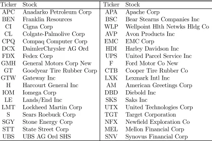
are reported in Appendix A.2). In "Test Group Dow Jones" (TGDJ) we include 30
Dow Jones Industrial Average index stocks that were decimalized on the decimalization
date, January 29, 2001 (see Table 1).9 They are typically much more active and have
7More precisely, in the quote data, we keep modes 1, 2, 3, 6, 10, and 12. In the trade data, we
exclude all other trades than the so-called regular trades. See the TAQ2 User Guide for details.
8We exclude AOL and TWX from the analysis because of their merger in January, 2001. On the
other hand, we keep DCX and UBS although they are American Depositary Receipts because Ahn, Cao, and Choe (1998)find that orderflows do not seem to migrate easily from market to market.
9Because MSFT and INTC are primarily Nasdaq stocks but part of the Dow Jones Industrial
larger market capitalization than the CG18 stocks. We thus decide to form another
test group called "Test Group 18" (TG18) in which we include 18 stocks of similar
activity to CG18. In order to improve the match between them, the TG18 stocks are
also pairwisely chosen from the same industry subsector or sector as the CG18 stocks
(see Table 2).10 Some descriptive statistics of all the stocks included in our analysis are
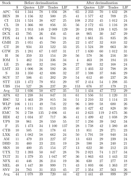
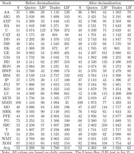
reported in Tables 3 (CG18 and TG18) and 4 (TGDJ).
Data errors are likely to be more frequent in UHF data than in sparsely sampled
data. With all the trades and quotes at our disposal, however, the errors are also easier
to detect. In the terminology of Aït-Sahalia, Mykland, and Zhang (2006), we say that
a midquote or trade price is a "bounceback" if a (logarithmic) return larger than a
prespecified threshold is followed by a return of similar magnitude but of opposite sign (so that the returns approximately cancel out). We use the following threshold rule:
for stocks priced below $10, in between $10 and $50, in between $50 and $100, and larger than $100 we set the threshold to 0.01, 0.0083, 0.0067, and 0.005, respectively. In the before decimalization period, we further multiply the thresholds by1.5for stocks trading in fractions (although this adjustment turns out to be insignificant). We find that in general there are more bouncebacks in the trade price data than in the midquote
data. This suggests that trade price data are inherently more noisy (bouncy). We delete
all found bouncebacks.
Bouncebacks can also be "sticky" in the sense that a data error can repeat for a
while. Sticky bouncebacks are much more of a problem in the midquote data than in
the trade price data. We detect them by comparing the return and the corresponding
spread to the daily standard deviation and spread, respectively. If the spread increases
only temporarily from its daily average and is followed by a midquote returning to its
previous level, a sticky bounceback is detected and deleted unless it is easy to correct
by PFE.
10One could match also with respect to other factors such as price, volatility, and equity market
for.11 These procedures detect the errors well.
When the sampling frequency gets high, the choice of data type becomes more
relevant. It is often argued that a midquote (defined as the average of the bid and ask quotes) provides a less noisy measure of the unobserved true price [see, e.g., Hasbrouck
(2007)]. On the NYSE, the variance of the market microstructure noise of midquote
returns actually partly reflects the bid-ask quote setting behavior of the specialists. For example, if the price of a stock suddenly moves significantly (up or down), the spread tends to widen momentarily (in the same direction) due to inventory positioning and
information asymmetry. In our analysis, we use both trade price and midquote data in
order to show how differently decimalization can affect them.12 We use the superscripts
"t" and "q" to denote their respective estimates.
The key statistical difference between midquotes and trade prices relevant to us is
that the first differences of midquotes do not typically have significant negative fi rst-lag autocorrelation commonly addressed to the bid-ask bounce [Roll (1984)], rounding
errors [Harris (1990a)], and inventory imbalances [e.g., Jegadeesh and Titman (1995)].
Instead, the midquote returns typically show significant positive autocorrelation for a few lags (and zero afterwards). While this is generally true, the strength of the
dependence can vary over time and across stocks [see Hansen and Lunde (2006) and
Curci and Corsi (2006)]. We find, for example, that the Ljung—Box (LB) test statistic is able to vary considerably between days and stocks. It tends to be stronger (weaker)
in midquote returns (trade price returns) after decimalization (see Tables 3 and 4). We
return to this issue in the next section where statistical tests are run. Furthermore, it
is not uncommon to observe other sort of autocorrelation patterns, especially for the
less active stocks such as the CG18 and TG18 stocks. The autocorrelation structure
also depends on the concept of time (the clock).
In our analysis, the clock is set in event time. Event time refers either to trade or
11We avoid deleting consecutive quotes because it leaves a gap in the durations between quotes.
Deleting consecutive quotes can be especially harmful for an inactive stock. Because it is sometimes hard to diagnose data errors correctly, the remainder becomes part of market microstructure noise.
12Naturally other types of data could be used as well, for example weighting the bid and ask quotes
quote time depending on the data type used. It is defined by taking each consecutive event (trade or quote) in consideration with equal weigth so that the distance between
two consecutive events is always one unit of time.13 This guarantees that no data
(information) is thrown away. This gives us an edge over the earlier decimalization
studies typically using the "old-school" way of sampling at equidistant calendar time
intervals (e.g., 1 min). It is nowadays also widely believed that calendar time sampling
is not very well-suited for the analysis of the evolution of a true price in liquid markets
[see, e.g., Frijns and Lehnert (2004)]. The problems of calendar time sampling arise from
the use of mandatory artificial price construction rules (e.g., interpolation between two prices) and from several well-known intraday patterns which tend to make the calendar
time sampled series non-stationary.
4
Empirical analysis
4.1
Preliminary analysis
We now descriptively evaluate the decimalization effects on volatility and market
mi-crostructure noise variance. We also demonstrate how well the non-parametric
esti-mators described above perform. This should facilitate the interpretation of the test
results in the next section.
We first find that the TSRV, GTSRV, MSRV, and RSRV estimators adapt quite naturally to different data types and concepts of time. The parametric methods
sug-gested in the literature [see, e.g., Aït-Sahalia, Mykland, and Zhang (2005a)] would not
be nearly asflexible. The parametric methods would, in particular, require us to take a stand on the structure and strength of the noise. This would complicate matters
considerably in an empirical study like ours where many stocks are analyzed. Although
the non-parametric volatility estimators we use are also quite robust to data errors, we
encourage some attention to be paid to the choice of time-scales that are being averaged
over. We next describe a setup which we found reasonable (although our results are
not sensitive to this setup).
The TSRV and MSRV estimates are calculated withK andM matching the number of quotes (trades) in 10 or 15 minutes on average, respectively. These choices may at
first seem arbitrary and as such to produce considerable amount of estimation error but as Aït-Sahalia, Mykland, and Zhang (2006) have shown, these two estimators are
quite robust in this sense. We have here merely tried to adjust the estimators to the
daily pace of the market without using any complicated optimality formulas. For very
active stocks, obviously,K andM can be much larger than for inactive stocks. Because this may cause problems for the least active stocks on slow days, we fix the lower limit to K = 10 if there are less than 10 observations in 10 minutes. We do not make any such adjustment to the MSRV estimator. For the GTSRV, we select J according to how strong the daily autocorrelation is: if the LB test statistic is greater than25 (the
chi-square5% critical value), then we useJ = 2 and5for the trade price and midquote data, respectively. These choices reflect the typical autocorrelation pattern for an active stock. If the daily autocorrelation is weak (LB is less than 25), then we use J = 1 (corresponding to the TSRV). We advice against using a too large J if the strength of the dependence does not call for it because this would cause underestimation.
Tables 5 and 6 report the average MSRVt(trade price data) estimates for each stock
before and after decimalization. The many downward pointing arrows suggest that
there is a general tendency for the volatility to be lower after decimalization. These
tables also show that although the MSRVtestimates are close to the MSRVq (midquote
data) estimates, the former are on average around4%above the latter regardless of the
period and stock group (see columns %q). On the other hand, the RVt estimates are
clearly inflated before decimalization and tend to become closer to the MSRVtestimates after decimalization (see columns %t
rv). For TGDJ, for which this effect is particularly evident, the reduction is from−174% to−26% implying only moderate overestimation
RVq estimates are deflated compared to the MSRVt estimates before decimalization. The noise reduction is also far less obvious than with the trade price data (see columns
%q
rv). Interestingly, for the inactive stocks the RVq estimates are actually close to the
MSRVq estimates in both periods (see Table 5).
The TSRV estimates do not show any clear tendency for over or underestimation
for the less active stocks (CG18 and TG18). For TGDJ, the TSRVtestimates are again
around 4% above the TSRVq estimates in both periods. The GTSRV estimates seem
to be more sensitive to the activity of the stock. This is probably due to the generic
choice of J which works better with the active than the inactive stocks. For example, for TGDJ, the trade price and midquote GTSRV estimates are on average very close to
each other (within1%margin), but for CG18 and TG18 the GTSRVtestimates tend to
be significantly lower than the GTSRVq estimates. (The TSRV and GTSRV estimates are reported in Appendix A.3.)
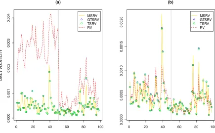
Figure 1 illustrates how the volatility estimators compare to each other in the case
of an active Dow Jones stock, Pfizer Inc. (PFE). The TSRV, GTSRV, and MSRV estimates are close to each other regardless of the data type used. On the other hand,
as seen in subplot (a), the RVt estimates are clearly inflated before the decimalization date but more in line with the others after it. In subplot (b) we see that the RVq
estimates are close to the other estimates in both periods and that the reduction due
to decimalization seems much less significant than the corresponding trade price data reduction.
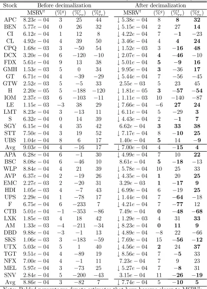
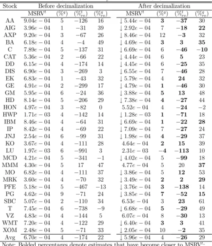
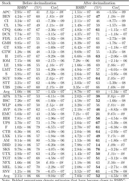
Tables 7 and 8 report the average RSRVt noise variance estimates. Again we see a
tendency for lower estimates after decimalization. The RSRVt estimates are above the
RSRVq estimates especially before decimalization (see columns %q). For TGDJ (Table
8), for example, the RSRVt estimates are on average 73% higher than the RSRVq
esti-mates before decimalization and 53% higher after decimalization. Decimalization thus
appears to have made the RSRV estimates closer to each other by decreasing the noise
more in the trade price data than in the midquote data. That the difference between
0 20 40 60 80 100 0 .000 0. 001 0. 002 0. 003 0. 004 (a) D A IL Y V O LA TI LI TY MSRV GTSRV TSRV RV
0 20 40 60 80 100
[image:20.612.81.516.49.318.2]0. 00 00 0. 0 005 0. 0010 0. 0015 0. 002 0 (b) MSRV GTSRV TSRV RV
Figure 1: Volatility of PFE using (a) trade prices; (b) midquotes. The last day of the before decimalization period is marked at observation #50 by the vertical line.
between the noise and the true volatility [see Hansen and Lunde (2006)]. In these
two tables we also report the first-lag autocovariance estimates for the noise variance. Except perhaps for TGDJ, however, they are dubious. Some of them actually imply
negative variances (the daily estimates even more often so). Thus in the subsequent
analysis we mainly rely on the RSRV estimates instead.
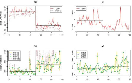
Figure 2 illustrates the associated changes in the noise variance and the SNR. The
decrease in the RSRVtestimates and the increase in the SNRt
3are obvious in subplots (a)
and (b). The changes are less apparent using the midquotes as can be seen in subplots
(c) and (d). In subplots (a) and (b) we have also included the first-lag autocovariance and the corresponding SNRt
3b estimates. The former are below the RSRVt estimates.
In fact, they are close to the RSRVq estimates, suggesting that the midquotes could be
used to reduce the upward biasedness of the trade price data estimates (see Tables 7
and 8). As a consequence, the SNRt
0 20 40 60 80 100 0e+ 00 2e-07 4e-07 6e-07 (a) N O ISE VAR IAN C E RSRV |COV(1)|
0 20 40 60 80 100
5. 0e-08 1. 5e-07 (c) RSRV
0 20 40 60 80 100
1000 3000 5000 (b) S IGN A L -T O-N O IS E SNR(3) SNR(2) SNR(1) SNR(3b)
0 20 40 60 80 100
2000 6000 10000 14000 (d) SNR(3) SNR(2) SNR(1)
Figure 2: Noise variance and SNR of PFE using trade prices (left panel) and midquotes (right panel). The solid black horizontal lines denote the mean of RSRV (upper panel) and SNR3 (lower panel). The vertical line at observation #50 denotes the last day of
the before decimalization period.
4.2
The test results
In this section, which contains the bulk of the results, we use the paired t-test for a group of non-independent samples in order to test whether the means of various
vari-ables were different from each other before and after thefinal decimalization date. The paired t-test is standardly applied in similar contexts including a few earlier decimal-ization studies [see, e.g., Bessembinder (2003)]. The test assumes that the differences
between the paired values are randomly drawn from the source population and that the
source population can be reasonably supposed to be normally distributed. However,
because normality of the differences is sometimes a too restrictive assumption, we also
use another standard test, namely the Wilcoxon rank sign test, which requires only
symmetry and not normality. The Wilcoxon rank sign test ranks the median values of
see, e.g., Hollander and Wolfe (1999)].14 Notice that serial dependence between
obser-vations (i.e., order) in the before and after decimalization periods is not relevant for
the calculation of these test statistics because only the differences between the
uncondi-tional means are used. And although the assumption of independence between the pairs
of stocks may be questioned (especially during big stock market downturns), we regard
it is as a reasonable assumption if the stocks are picked in random from different sectors
as they essentially now are (see Section 3). Also, the stocks within each group CG18,
TG18, and TGDJ are much alike in trading activity which makes taking averages over
them less of a problem than if they would not have anything in common.
Wefirst report the paired t-test and the Wilcoxon rank sign test results for the ab-solute and relative spread, number of quotes and trades, quoted depth, trading volume,
and serial dependence. This helps us to interpret the main results on volatility and
market microstructure noise variance (reported next). Our findings can be compared to the earlier studies with some precautions in mind, mostly related to different market
mechanisms (see Section 1).
From Table 9 we see that, for CG18, none of the seven variables change significantly except the number of quotes which increases over the two periods (not abruptly but
smoothly). In particular, wefind no significant changes in the number of trades, trading volume (in round-lots), or LB test statistics (for 15 lags). Thus the control group is
largely unaffected by the decimalization of the other stocks as it ideally should. In
contrast, most of the variables for TG18 and TGDJ change significantly. As expected, we find a significant decrease in their quoted depth and a very significant decrease in their spreads. TGDJ has no significant increase in the number of quotes but TG18 does. This is probably due to the fact that the quotes for the most active stocks were already
updated frequently before the decimalization date. Interestingly, for both TG18 and
14The paired t-test is calculated as (X −Y)/S.E.[(X −Y)], where the denominator is the
stan-dard error of the difference of the two averages. Notice that the nominator is numerically equivalent with calculating the average of the paired differences. The Wilcoxon rank sum test is calculated as
Pn
TGDJ, the midquote return autocorrelation tends to increase. In contrast, the trade
return data autocorrelation decreases, although both groups have a significant increase in the number of trades. The decrease is more significant for TGDJ, again probably due to its higher activity. A decrease in the first-lag autocorrelation is in line with theory that predicts less significantfirst-lag autocorrelation due to smaller rounding error [see Harris (1990a)]. That the number of trades increases for both TG18 and TGDJ while
their trading volume stays constant is also in line with the earlier studies.
From Table 10, on the other hand, we see that the midquote absolute first-lag covariances decrease or do not change at all. Because the corresponding LB test statistic
was just found to increase (see Table 9), decimalization seems to have weakened the
first-lag dependence but strenghtened the higher lag dependence. This would explain the apparent controversy between the LB of midquote and trade data (although this is
stock dependent to some extent as noted above). The main reason why the dependence
should be increased in the midquote data is, we believe, that decimalization changed the
strategic behavior of the market participants. The participants outside the "floor" of the NYSE may have for example become more cautious due to the fear of "front-running"
(a form insider trading from the part of the NYSE specialists). This is consistent with
the reported decrease in market transparency [see, e.g., NYSE (2001)]. In general,
the simple and significantly weakened serial dependence in the trade price data should make them better suited for the analysis of decimalization effects than the midquote
data especially with the most active stocks.
We now turn to our main results that are reported in Table 10. According to the
paired t-test, true volatility appears to decrease only slightly (CG18 and TGDJ) or not significantly (TG18). The Wilcoxon test provides much stronger evidence of a decrease which is evidently due to the non-Gaussian character of volatility. The results
also reveal that there are in general only minor differences between the three volatility
estimators we use. The MSRV estimates indicate a slightly more significant decrease for TGDJ (whether this may be due to jumps is discussed in the next section). Noise
decrease in noise variance turns out to be more significant than the volatility decrease. Not surprisingly, then, the increase in their SNR is highly significant for TGDJ. We
find no major differences between SNR1, SNR2, and SNR3 but SNR3 changes slightly
less significantly than the others.
Notice that the results using trade price data (left panel in Table 10) differ in some
respects from the midquote data results (right panel). The trade price data tend to
give slightly more significant results than the midquote data for the volatility of TGDJ. The difference is more obvious for the noise variance. As a consequence, the increase
in SNRt for TGDJ turns out to be highly significant. The data type does not seem to matter as much for TG18, however, suggesting that the less active stocks are less
affected by the data type.
It is of course possible that the tests applied here accidentally capture inherent
trends in the data and, in the case of volatility in particular, clustering to turbulent
and tranquil times that are not related to the decimalization process itself. As a first attempt to control for confounding factors, we run linear regressions for each stock
with volatility, noise variance, and SNR as the dependent variables. The explanatory
variables we use are the number of quotes (for the midquote data) and trades (for the
trade price data), the LB test statistic, and a dummy variable defined to be 0 before decimalization and 1 after it. The number of quotes and trades are included because
they appear prominently in the calculation of the estimates (see Section 2) and because
they have not, in general, remained constant over the sample period (see Table 9). The
LB test statistic, on the other hand, is included because it can be thought as reflecting the daily information asymmetry and because it has not in general remained constant
either. Note that we do not include the spreads as explanatory variables because they
correlate highly with the dummy variable for the TGDJ stocks. Multicollinearity could
easily lead to invalid inference regarding the regression coefficients. Such approximate
multicollinearity actually only supports the view that the most active stocks had the
largest spread and noise variance reductions.
signif-icantly negative when the dependent variable is either volatility or noise variance. So
confounding factors do not appear to be responsible for the decrease. It is however
harder to tell what the effect on the SNR is because the corresponding dummy coeffi
-cient is often close to zero and its sign alternates stock dependently within and between
groups. In order to gain more insight, we run panel (longitudinal) linear regressions
with the same dependent and explanatory variables. Specifically, we use the restricted maximum likelihood method to estimate linear mixed-effects models of the form [see
Pinheiro and Bates (2004, Ch. 2)]
yit = α+β1LB(15)it+β2NrT rades(Quotes)it+β3Dummyit+
ai+b1iLB(15)it+b2iNrT rades(Quotes)it+b3iDummyit+ it,
where i denotes the ith stock in CG18/TG18 (i = 1, ...,18) or TGDJ (i = 1, ...,30) and t denotes the day before and after decimalization (t = 1, ...,98). Here α and βh (on the top row) are the fixed-effect coefficients and ai and bhi (on the bottom row) are the random-effect coefficients. The latter describe the shift in the intercept and the
explanatory variables for each stock, respectively, and they are assumed to be normally
distributed with mean zero. The random-effect coefficients are allowed to be correlated
(with a covariance matrix not depending on the stock) but the normally distributed
and zero-centered error terms it are assumed to be independent. Thus, the random
effects can be regarded as additional errors terms that account for correlation among
observations (for each stock separately).
The trade price and midquote data panel regression results are reported in Tables 11
and 12. In them, volatility is estimated by the MSRV (the other estimators would do as
well). In order to facilitate interpretation of the regression coefficients and to mitigate
multicollinearity, we center the explanatory variables except the dummy. As seen above,
we include random effects for all the explanatory variables including the dummy. This
significant when volatility and noise variance are dependent variables. However, there does not appear to be much support for a significant abrupt increase in the SNR: after controlling for the number of quotes and trades, in particular, the coefficient for the
dummy turns out to be insignificant or of the wrong sign (midquote data) or to be only mildly significant (trade price data). Specification tests done along the lines of Pinheiro and Bates (2004, Ch. 4.3) do not reveal any clear evidence of misspecifation — especially
when random effects are included for everyfixed-effect explanatory variable as they now are. In particular, we then find that the standardized within-stock residuals are zero centered and normally distributed.
We conclude that after taking confounding and random effects into account, at best
only weakly significant evidence of an abrupt level shift in the SNR exists and that only the trade price data provide evidence in favor of an increase. The last point makes
sense because the trade price data are more sensitive to the change in the tick size.
In fact, if the midquotes correctly represent the true price, the corresponding dummy
should not be significant. Of course, we cannot totally exclude the possibility that the above findings are not due to the relatively short sample period in question. However, longer periods or periods farther apart from each other would potentially suffer even
more from trends and complicate the inference.
4.3
The e
ff
ect of jumps
It is a well-known theoretical fact that if jumps exist, RV does not converge to IV
even in the absence of market microstructure noise but instead toIV+P0≤t≤T |∆Xt|2, where∆X denotes a large return (a true jump triggered by an earnings announcement, for example). It has also been reported that estimators such as the TSRV and MSRV
then lose part of their estimation accuracy [see Fan and Wang (2006)]. This has raised
some doubts about the validity of earlier research [see, e.g., Diebold (2005)]. We thus
next study if jumps exist in our data and if the jumps affect our results on
discrete data, we also pay some attention to how much noise there is in the trade price
data compared to the midquote data.
Wefirst test for the presence of jumps. For this purpose we use the test proposed by Aït-Sahalia and Jacod (2006) which we call the two-scale jump test (TSJT). This test
is valid only in the absence of market microstructure noise so we expect to see some
bias, but we nevertheless find it useful to calculate for qualitative purposes. The good thing is that the TSJT is a particularly direct and easy way to test for the presence of
jumps (but not their strength or frequency) without making strong assumptions. We
now shortly review it.
The TSJT statistic is defined as
b
S(p, k,∆n)t= b
B(p, k∆n)t b
B(p,∆n)t
,
where, forp >0,
b
B(p,∆n)t:=
[t/X∆n]
i=1
|∆niX|p
is the estimator of variability, and ∆n
iX = Xi∆n −X(i−1)∆n denote the discrete incre-ments of a semimartingale process X. As is easily observed, the TSJT statistic takes advantage of two overlapping time-scales,∆n andk∆n,from which we have derived its name.
The usefulness of this test is based on a theorem in Aït-Sahalia and Jacod (2006)
saying that if t > 0, p > 2, and k ≥ 2, then the variables Sb(p, k,∆n)t converge (in probability) to the variable S(p, k)t = 1 on the set of discontinuous processes and to
kp/2−1 on the set of continuous processes as∆
n → 0 (n→ ∞). Aït-Sahalia and Jacod (2006) show that if the market microstructure noise is IID and p= 4, then the TSJT statistic converges to1/k(instead of1).They note, however, that whenE 2 andE 4 are
small (as in practice they are; see for exampledE 2 in Tables 7 and 8) and∆
n =T /nis "moderately small," then the TSJT statistic will again be close to1in the discontinuous
We use the values p = 4 and k = 2 and set [0, T] to one trading day as suggested by Aït-Sahalia and Jacod (2006). We let ∆n to vary from 1 to 10 events but report here only the results with ∆n = 1 (the larger time-scales give less accurate results).
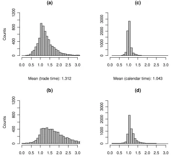
The non-normalized histograms of all the stocks together are presented in Figure 3.
There are 6 468 observations in total, each observation representing one day for one
stock. The subplots (a) and (b) indicate that market microstructure noise is prominent
because the histograms are not tightly peaked around any value. In particular, the
histograms are not centered around 1 or 2. The mean of the midquote data is higher
than the mean of the trade price data. This is in line with the view that the midquote
data are less bouncy than the trade price data (see Section 3).15
For comparison purposes, in subplots (c) and (d) we show the histograms in calendar
time with ∆n = 5 seconds. These histograms are more sharply centered around 1,
implying more jumpy price evolution or less noise contamination in calendar time.
Both explanations are in fact plausible.16 The price process may be more jumpy in
calendar time because the price does not adjust instantly to new surprising news. This
would be consistent for example with the idea of subordination and the directing process
evolving at different rates [see, e.g., Clark (1973)]. In event time the jumps also tend
to be smoothed out by market makers who monitor the market closely. The fact that
the histograms of trade price and midquote data look more like each other in calendar
than in event time supports the view that the data type plays a less significant role in larger time-scales (and with less active stocks).
There are at least two straightforward ways to remove jumps [see Barndorff-Nielsen
and Shephard (2004) and Aït-Sahalia and Jacod (2006)]. Both of these methods (as
they currently stand), however, work well only in the absence of market microstructure
noise. Thus we decide to apply the following simple rule instead: if the return of
consecutive prices in event time is larger than a given threshold (we use0.03), then the
15It would not make sense to call the trade price data truly more jumpy than the midquote data
because both data types reflect the same underlying value.
16Aït-Sahalia and Jacod (2006)find their histogram to be centered below 1. They however include
(a)
Mean (trade time): 1.312
Co
un
ts
0.0 0.5 1.0 1.5 2.0 2.5 3.0
0 4 0 0 800 1 200 (b)
Mean (quote time): 1.772
Co
un
ts
0.0 0.5 1.0 1.5 2.0 2.5 3.0
0 4 0 0 80 0 1 20 0 (c)
Mean (calendar time): 1.043
0.0 0.5 1.0 1.5 2.0 2.5 3.0
0 10 00 20 00 3000 (d)
Mean (calendar time): 1.149
0.0 0.5 1.0 1.5 2.0 2.5 3.0
[image:29.612.114.470.51.383.2]0 1000 20 00 30 00
Figure 3: Histograms of the TSJT statistic in event time using (a) trade prices; (b) midquotes. Subplots (c) and (d) show the corresponding data in calendar time.
return is removed, a new price table is constructed, and the statistical tests are re-run.
This reduces the daily number of quotes and trades but only slightly because so big
jumps are quite rare in event time. In fact, there are only a few such jumps in each
group per period and less in the midquote data than in the trade price data. Of course,
the number of jumps would be greatly increased if we would use a smaller threshold
but then we would also be more likely to capture not only the true jumps but also
noise. This would be especially true with the less active CG18 and TG18 stocks. For
completeness, we report the number of jumps with three different thresholds in Tables
13 and 14 which clearly show the increase in the number of jumps when the threshold
Because most of the days do not have any significant jumps according to the above threshold (0.03), the sums of power 4 stay largely unaffected when the jumps are re-moved. We see no obvious differences between the before and after period either. The
paired t-test statistics are only moderately affected by the jumps (and the Wilcoxon test less so). The change is most evident for volatility and noise variance; in the case of
a low priced stock, a big price swing can make jumps more likely in one of the periods
and thus produce many jumps (see, e.g., LU in Table 4). But even in this case the
effect on the SNR is diminishingly small because both the noise variance and the true
volatility decrease by approximately the same amount. So we conclude that jumps do
not seem to have any qualitatively important impact on our results. This seems like
a natural result as true jumps are basicly randomly scattered over time independently
of the decimalization process and the test statistics we use group many practically
independent (although similar in trading activity) stocks together.
5
Conclusions
In this paper we have empirically studied the effect of decimalization on volatility and
market microstructure noise using UHF data. A key point is to estimate the true
volatility accurately. To this end, we have used three non-parametric estimators that
all have desirable statistical properties and are yetflexible and simple to calculate. We have estimated the market microstructure noise variance non-parametrically as well.
Statistical tests are run in order to evaluate the significance of the effects on volatility, noise variance, and their ratio.
The main result of this empirical study is that decimalization decreased observed
volatility by reducing noise variance especially for the highly active stocks. The
reduc-tion can be attributed to smoother price evolureduc-tion or, in other words, to diminished
price discreteness. Consequently, the significance of the true signal appears to have in-creased. Mixed-effect panel regression results show, however, that most of this increase
results than the midquote data which is in line with the view that trade prices are more
sensitive to the changes in the tick size and that they provide a less accurate estimate
of the true (unobserved) price. For the inactive stocks the difference between the two
data types appears to be insignificant.
It should be noted, however, that the decrease in observed volatility due to
decimal-ization can be slightly deceptive. As the markets also became less transparent and the
market making costs increased, algorithmic trading gained more popularity in so much
that it nowadays makes up a big portion of the daily volume. In a crisis, algorithmic
trading can lead to sell-offpressures that may actually end up increasing volatility in
the decimal regime.
This study also demonstrates how the TSRV, GTRSV, and MSRV estimators
per-form in a changing environment. The MSRV estimator appears to give the most robust
estimates with respect to the data type and tick size used. This is noteworthy because
wefind that decimalization decreased linear dependence in the trade data but increased it in the midquote data. On the other hand, the MSRV trade price data estimates are
on average a few percents higher than the respective midquote data estimates in both
periods. This discrepancy may be due the fact that the MSRV estimator does not
adjusting to all complex dependencies. Nevertheless, we feel that the non-parametric
volatility estimators used here can be considered as more flexible than the parametric estimators suggested in the literature.
Although the estimators we use are sensitive to jumps to certain extent (the volatility
estimators less than the RSRV), we do notfind true jumps to be critical for our results. Prefiltering the data for errors seems far more important because compared to jumps triggered by news, the errors tend to be bigger, more frequent, more systematic, and
harder to correct for especially in the quote data.
Finally, we note that the estimators we have used are accurate only in ideal
con-ditions that may not exist in practice over time and across stocks. We feel that there
is room for improvement especially in the estimation of noise variance by taking more
decom-pose volatility into even smaller components. Separating small components from each
other would make the effect of decimalization even more transparent. Decomposition of
market microstucture noise would however require us to take a stand on questions such
as what constitutes a jump and how to separate it from other noise sources. This is a
topic of both theoretical and practical interest and likely to become more important as
References
Aït-Sahalia, Yacine, and Jean Jacod. (2006). "Testing for Jumps in a Discretely Ob-served Process." Working Paper, Princeton University and UPMC.
Aït-Sahalia, Yacine, Per A. Mykland, and Lan Zhang. (2005a). "How Often to Sample a Continuous-Time Process in the Presence of Market Microstructure Noise." Review of Financial Studies 18, 351—416.
–– (2005b). "Comment on ’Realized Variance and Market Microstructure Noise’ by Peter Hansen and Asger Lunde." Technical Report, University of Chicago.
–– (2006). "Ultra High Frequency Volatility Estimation with Dependent Microstruc-ture Noise." Working Paper, Princeton University, University of Chicago, and Univer-sity of Illinois.
Ahn, Hee-Joon, Charles Q. Cao, and Hyuk Choe. (1996). "Tick Size, Spread, and Volume." Journal of Financial Intermediation 5, 2—22.
–– (1998). "Decimalization and Competition Among Stock Markets: Evidence from the Toronto Stock Exchange Cross-Listed Securities."Journal of Financial Markets 1, 51—87.
Amihud, Yakov, and Haim Mendelson. (1987). "Trading Mechanisms and Stock Re-turns: An Empirical Investigation." Journal of Finance 42, 533—553.
Bacidore, Jeffrey M. (1997). "The Impact of Decimalization on Market Quality: An Empirical Investigation of the Toronto Stock Exchange." Journal of Financial Inter-mediation 6, 92—120.
Bacidore, Jeff, Robert Battalio, and Robert Jennings. (2001). "Changes in Order Char-acteristics, Displayed Liquidity, and Execution Quality on the New York Stock change Around the Switch to Decimal Pricing." Working Paper, New York Stock Ex-change.
–– (2003). "Order Submission Strategies, Liquidity Supply, and Trading in Pennies on the New York Stock Exchange."Journal of Financial Markets 6, 337—362.
Bandi, Federico M., and Jeffrey R. Russell. (2003). "Microstructure Noise, Realized Volatility, and Optimal Sampling." Working Paper, University of Chicago.
–– (2006). "Separating Microstructure Noise from Volatility." Journal of Financial Economics 79, 655—692.
Barndorff-Nielsen, Ole E., and Neil Shephard. (2004). "Power and Bipower Variation with Stochastic Volatility and Jumps."Journal of Econometrics 2, 1—37.
Bessembinder, Hendrik. (2003). "Trade Execution Costs and Market Quality after Dec-imalization."Journal of Financial and Quantitative Analysis 38, 747—778.
Bollen, Nicolas P. B., and Robert E. Whaley. (1998). "Are Teenies’ Better?" Journal of Portfolio Management 25, 10—24.
Chakravarty, Sugato, Robert A. Wood, and Robert A. van Ness. (2004). "Decimals and Liquidity: A Study of the NYSE."Journal of Financial Research 27, 75—94.
Chakravarty, Sugato, Venkatesh Panchapagesan, and Robert A. Wood. (2005). "Did Decimalization Hurt Institutional Investors?"Journal of Financial Markets 8, 400—420.
Chakravarty, Sugato, Bonnie F. van Ness, and Robert A. van Ness. (2005). "The Effect of Decimalization on Trade Size and Adverse Selection Costs." Journal of Business Finance and Accounting 32, 1063—1081.
Cho, D. Chinhyung, and Edward W. Frees. (1988). "Estimating the Volatility of Dis-crete Stock Prices." Journal of Finance 43, 451—466.
Chung, Kee H., Bonnie F. van Ness, and Robert A. van Ness. (2004). "Trading Costs and Quote Clustering on the NYSE and NASDAQ After Decimalization." Journal of Financial Research XXVII, 309—328.
Clark, Peter K. (1973). "A Subordinated Stochastic Process Model with Finite Variance for Speculative Prices."Econometrica 41, 135—155.
Curci, Giuseppe, and Fulvio Corsi. (2006). "Discrete Sine Transform for Multi-Scales Realized Volatility Measures." Working Paper, Universita di Pisa and University of Lugano. Available at SSRN: http://ssrn.com/abstract=650504.
Diebold, Francis X. (2005). "On Market Microstructure Noise and Realized Volatility." Working Paper, University of Pennsylvania.
Easley, David, and Maureen O’Hara. (1992). "Time and the Process of Security Price Adjustment." Journal of Finance 47, 577—605.
Economist. (2007a). "Dodgy Tickers; Stock Exchanges."Economist, March 10, 2007.
Economist. (2007b). "Ahead of the Tape; Algorithmic Trading." Economist, June 23, 2007.
Engle, Robert F., and Zheng Sun. (2005). "Forecasting Volatility Using Tick by Tick Data." Working Paper, New York University. Available at SSRN: http://ssrn.com/abstract=676462.
Fan, Jianqing, and Yazhen Wang. (2006). "Multi-Scale Jump and Volatility Analysis for High-Frequency Financial Data." Working Paper, Princeton University and University of Connecticut.
Figlewski, Stephen. (1997). "Forecasting Volatility." Financial Markets, Institutions, and Instruments 6, 1—88.
Gibson, Scott, Rajdeep Singh, and Vijay Yerramilli. (2003). "The Effect of Decimaliza-tion on the Components of the Bid-Ask Spread."Journal of Financial Intermediation
12, 121—148.
Goldstein, Michael A., and Kenneth A. Kavajecz. (2000). "Eigths, Sixteenths, and Market Depth: Changes in Tick Size and Liquidity Provision on the NYSE." Journal of Financial Economics 56, 125—149.
Gottlieb, Gary, and Avner Kalay. (1985). "Implications of the Discreteness of Observed Stock Prices." Journal of Finance 40, 135—153.
Glosten, Lawrence R., and Paul R. Milgrom. (1985). "Bid, Ask, and Transaction Prices in a Specialist Market with Heterogenously Informed Traders." Journal of Financial Economics 14, 71—100.
Griffin, Jim E., and Roel C. A. Oomen. (2006). "Sampling Returns for Realized Variance Calculations: Tick Time or Transaction Time?" Working Paper, University of Warwick. Available at SSRN: http://ssrn.com/abstract=906472.
Hansen, Peter R., and Asger Lunde. (2006). "Realized Variance and Market Microstruc-ture Noise." Journal of Business and Economic Statistics 24, 127—161.
Harris, Lawrence. (1990a). "Estimation of Stock Price Variances and Serial Correlations from Discrete Observations."Journal of Financial and Quantitative Analysis 25, 291— 306.
–– (1990b). "Statistical Properties of the Roll Serial Covariance Bid/Ask Spread Estimator." Journal of Finance 45, 579—590.
–– (1991). "Stock Price Clustering and Discreteness."Review of Financial Studies 4, 389—415.
–– (1994). "Minimum Price Variations, Discrete Bid-Ask Spreads, and Quotation Sizes."Review of Financial Studies 7, 149—178.
–– (1997). "Decimalization: A Review of the Arguments and Evidence." Working Paper, University of Southern California.
–– (1999). "Trading in Pennies: A Survey of the Issues." Working Paper, University of Southern California.
Hasbrouck, Joel. (1996). "Modeling Market Microstructure Time Series." In G. Mad-dala, and C. Rao (eds.), Handbook of Statistics 14, North Holland, Amsterdam, pp. 647—692.
–– (2007). Empirical Market Microstructure Theory: The Institutions, Economics, and Econometrics of Securities Trading. Oxford University Press.
He, Yan, and Chunchi Wu. (2005). "The Effects of Decimalization on Return Volatility Components, Serial Correlation, and Trading Costs." Journal of Financial Research