Munich Personal RePEc Archive
Knowledge spillovers and total factor
productivity. Evidence using a spatial
panel data model
Fischer, Manfred M. and Scherngell, Thomas and Reismann,
Martin
Vienna University of Economics and Business, Austrian Institute of
Technology, Vienna University of Economics and Business
February 2008
Online at
https://mpra.ub.uni-muenchen.de/77762/
Knowledge spillovers and total factor productivity.
Evidence using a spatial panel data model
Manfred M. Fischer, Thomas Scherngell and Martin Reismann
Institute for Economic Geography and GIScience Vienna University of Economics and BA, Vienna, Austria
Abstract. This paper investigates the impact of knowledge capital stocks on total
factor productivity through the lens of the knowledge capital model proposed by Griliches (1979), augmented with a spatially discounted cross-region knowledge spillover pool variable. The objective is to shift attention from firms and industries to regions and to estimate the impact of cross-region knowledge spillovers on total factor productivity (TFP) in Europe. The dependent variable is the region-level TFP, measured in terms of the superlative TFP index suggested by Caves, Christensen and Diewert (1982). This index describes how efficiently each region transforms physical capital and labour into output. The explanatory variables are internal and out-of-region stocks of knowledge, the latter capturing the contribution of cross-region knowledge spillovers. We construct patent stocks to proxy regional knowledge capital stocks for N=203 regions over the
1997-2002 time period. In estimating the effects we implement a spatial panel data model that controls for the spatial autocorrelation due to neighbouring regions and the individual heterogeneity across regions. The findings provide a fairly remarkable confirmation of the role of knowledge capital contributing to productivity differences among regions, and add an important spatial dimension to the discussion, by showing that productivity effects of knowledge spillovers increase with geographic proximity.
Keywords. Total factor productivity, knowledge spillovers, European regions,
panel data, spatial econometrics
JEL Classification. C23, O49, O52, R15
Revised February 2008
Correspondence: Manfred M. Fischer, Chair for Economic Geography, Institute for Economic Geography &
2 1 Introduction
Many economic studies, such as the pioneering study by Solow (1957), have demonstrated the
central role played by technological progress in economic growth. These studies based on a
growth-accounting approach do not attempt to measure technological progress directly, but treat
it as the residual factor accounting for growth. According to the standard interpretation, this
residual represents disembodied technological progress, usually referred to as total factor
productivity (TFP), defined as output per unit labour and physical capital combined.
This paper lies in the research tradition that investigates the impact of knowledge capital stocks
on total factor productivity through the lens of the knowledge capital model proposed by
Griliches (1979) to augment the production function with the stock of knowledge1. The knowledge capital model has become the cornerstone of the productivity literature for more than
25 years and has been applied in dozens of empirical studies on firm-level productivity and
extended to the more aggregated industry- and country-levels (see Griliches 1995 for a survey).
This model has evolved in many directions. Jaffe (1986) initiated ways of accounting for the
appropriability of external flows of knowledge or knowledge spillovers. Knowledge spillovers
may be defined to denote the benefits of knowledge to firms, industries or regions not
responsible for the original investment in the creation of this knowledge. It is important to
distinguish between two distinct types of knowledge spillovers: Spillovers embodied in traded
capital or intermediate goods and services (so-called pecuniary externalities)2 and spillovers of the disembodied kind (non-pecuniary externalities). The focus of this paper is on spillovers of
the second type. Such spillovers arise because the production of knowledge has public good
characteristics limiting the ability of firms to stop other firms or individuals exploring it.
1 It is worth emphasizing that this field is rather different from the abundance of studies that aim to estimate a
knowledge production function that relates the output of the knowledge production process, the increment of economically valuable technological knowledge in a region, to R&D inputs. Regional knowledge production is seen to depend on two major sources: university research and commercial R&D (see, for example, Anselin, Varga and Acs 1997; Fischer and Varga 2003). Such knowledge production function studies allow for testing hypotheses about the impact of spillovers from academic research and about the existence of Jacobian spillovers, and permit statements about the spatial extent of knowledge externalities but no statements about productivity effects.
2 As pointed out by Griliches (1995), pecuniary externalities that work through the price system are not really a
3
The last few years have seen the development of a significant body of research that includes
measures of external knowledge capital in an attempt to estimate the productivity effects of
knowledge spillovers across firms (see, for example, Los and Verspagen 2000, and Mairesse and
Sassenou 1991 for a survey), across industries (see, for example, Scherer 1993, and Branstetter
2001) or across countries (see, for example, Park 1995)3. Even though the subnational region is increasingly regarded as an important level of economic policy, there have been very few
attempts so far to investigate the impact of knowledge capital stocks on region-level total factor
productivity. One notable exception is the study by Robbins (2006) which finds mixed evidence
in terms of the significance of industry-specific knowledge spillovers at the state level in the US,
and a lack of evidence in most manufacturing industries. This contradicts the strong findings in
firm-level, sectoral and country-level studies.
The objective of our study is to investigate whether knowledge spilling across regional
boundaries has an impact on regional total factor productivity in manufacturing industries in
Europe. By Europe we mean the 15 pre-2004 EU member states. We use a panel of 203 NUTS-2
regions to estimate the spillover impact over the period 1997-2002. NUTS-2 regions are
interesting units of analysis in an increasingly integrated European market. They are more
homogeneous than countries, better connected within themselves, and they are becoming
increasingly important as policy units for research and innovation (see European Commission
2001).
3 It is worth noting that Coe and Helpman (1995) use weights related to input purchase flows to measure the impact
4
In using patent stocks4 to proxy knowledge stocks, we build on Robbins (2006), but depart from this previous work at least in two major aspects. First, we extend the knowledge capital model
with a spatially discounted cross-region knowledge spillover pool variable that allows to
measure rather than to assume the degree of localization of such spillovers, and second, we
account for spatial error autocorrelation due to neighbouring regions and the individual
heterogeneity across regions in estimating the model and, hence, avoid misspecification
problems.
The remainder of this paper is organized as follows. The section that follows presents the
reduced-form model that relates regional TFP not only to region-internal knowledge capital but
also to cross-region knowledge spillovers. We use a region-level relative TFP index – suggested
by Caves, Christensen and Diewert (1982) – as an approximation to the true TFP measure and
patent stocks to proxy regional knowledge capital stocks. Section 3 details the definition of the
TFP index and the construction of the regional patent stocks. Important econometric issues
raised by the estimation of the model are addressed in Section 4, while Section 5 reports the
estimation results. Section 6 concludes the paper.
2 The empirical model
The model used in this paper builds on the knowledge capital model (see Griliches 1979,
Doraszerlski and Jaumandreu 2008), but modifies it so that the region’s total factor productivity
depends not only on its own knowledge capital stock, but also on the level of the pool of general
knowledge accessible to it. Denote regions by i=1,...,N and time periods by t=1,...,T .
Ignoring constants, time trends or year dummies, the regional production function is given by
4 An alternative, widely used in firm-level studies, would be to use measures of R&D input. One problem with this
5
( , )
it it it it
Q =A g L C (1)
where g(.,.) is assumed to be homogeneous of degree one and to exhibit diminishing marginal returns to the accumulation of each factor alone. C is the stock of physical capital, L the stock of
labour, Q value added, and A an index of the technical efficiency of production with
( , )
it it it
A = A K K∗ (2)
where K and K∗ are the stocks of region-internal and region-external knowledge capital,
respectively. The stocks of knowledge capital are proxies for the state of knowledge. The knowledge created by a private or public agent is added to the pool of the existing knowledge capital stock to which other agents have access. Note that even if the benefits of R&D activities are fully appropriated by an agent, in the sense that an agent acquires a monopoly right by patent protection, some portion of the knowledge that has led to the patent may diffuse across regions through various communication channels such as publications, seminars, personal contacts, reverse engineering, (informal) exchange in networks, transfer of human capital and other means (Park 1995).
In an N-region world, the global stock of knowledge capital is given by
1
N
jt j
K
=
∑
(3)where the subscript j denotes the jth region, and knowledge capital Kjt is assumed to accumulate
with knowledge production activities and to depreciate from period to period at a rate rK. Hence,
its law of motion can be written as
1
1 1 1
1
(1 ) 1 jt
jt K jt jt jt K
jt
S
K r K S K r
K
−
− − −
−
⎛ ⎞
= − + = ⎜⎜ − + ⎟⎟
6
This law implies that knowledge production activities Sjt−1 undertaken in period t–1 become
productive in period t.
For region i, Kit represents its own knowledge capital stock in period t and Kit∗ its relevant pool
of knowledge spillovers. Since not all knowledge capital will necessarily spill over from one
region to another, it seems appropriate to define Kit
∗ as5
N
it ij jt m
j ì
K∗ w K −
≠
=
∑
(5)where wij represents region’s i ability to internalize pieces of region’s j knowledge stock for
production in region i, and Kjt m− represents the knowledge capital stock of region j at time t–m
(m positive integer).
The term w Kij jt m− may be interpreted as the effective fraction (pool) of the stock of knowledge
in region j “borrowed” by region i. The time lag is important since it takes time for knowledge
spillovers from region j to be expressed in new products and processes in region i. We construct
a spatially discounted time-lagged pool by assuming that the effective knowledge contribution
by each of the regions j (j≠i) depends on the geographic distance between that region j and
region i. This is quite in line with the literature on spatial knowledge spillovers (see Döring and
Schellenbach 2006 for a survey). Empirical work by Jaffe, Trajtenberg and Henderson (1993),
for example, on patent citations proxying knowledge spillovers showed the spatial decay in
knowledge spillovers relative to the patent source, which was interpreted as knowledge diffusion
decay. This motivated us to follow Fischer, Scherngell and Jansenberger (2006) in assuming a
parametric exponential dependence between weights and geographic distance as given by6
5 The definition shows that one faces two major problems in constructing the relevant pool of knowledge spillovers,
deciding on the appropriate time lag structure m and finding an appropriate weight structure { ,w iij ≠ j} to
represent borrowed knowledge and spillovers.
6 This exponential specification is attractive because of its theoretical underpinning in spatial interaction theory and
7
exp( )
ij ij
w = −δd (6)
which enables us to test rather than to assume the strength of the spatial dependence. dij denotes
geographic distance, in some sense, between the knowledge spilling region j and the knowledge
receiving region i. δ is the distance sensitivity parameter that captures the impact of distance on
the spillover variable. Estimating δ =0 would mean that distance would not matter. Positive
-estimates
δ would suggest that the benefits from out-of-region knowledge capital stocks exponentially decline with distance. Different distance measures can be used to represent
possible geographic impediments to the free flow of knowledge across space. In the context of
our study we measure distance between regions i and j as great circle distance between their
economic centres7.
Substituting Equation (2) into Equation (1) and assuming a Cobb-Douglas production technology
gives, for region i,
*
1 2 1
( , , , ) exp( )
it it it it it it it it it it
Q =Q K K L C∗ =Kγ K γ L Cα −α ε (7)
where α, 1−α γ γ, ,1 2 are the output elasticities with respect to labour, physical capital,
region-internal and region-external knowledge capital. ε is the error term reflecting all unmeasured
determinants of output and productivity, approximations and other disturbances.
Define total factor productivity F in the usual way as Fit =Qit/ (L Cαit it1−α) then it is easy to see
how total factor productivity is linked to knowledge stocks inside and outside the region in
question:
exp(−δdij) equals exp(−δdji). When dij equals zero, exp(−δdij) equals one. As dij approaches infinity,
exp(−δdij) approaches zero.
7 Travel distance is an alternative measure (see, for example, Crescenzi, Rodríguez-Pose and Storper 2007, LeSage
8
1 2 1 2 log exp ( )
N
it it it it it ij jt m it
j i
f γ k γ k∗ ε γ k γ δd K − ε
≠
⎡ ⎤
= + + = + ⎢ − ⎥+
⎣
∑
⎦ (8)where we follow the convention that lower case letters denote logs and upper case letters levels,
that is fit =logFit, logkit = Kit and kit logKit
∗ = ∗. Equation (8) is a simple panel data regression
model, where i denotes the cross-section and t the time series dimension. γ1 measures the effect
of the region’s own knowledge capital stock on total factor productivity, while γ2 captures the
relative effect from cross-region knowledge spillovers. A positive and significant estimate of γ2
is interpreted as evidence of such spillovers. For δ >0, variation in regional productivity levels
is best accounted for by giving a lower weight to knowledge capital stocks in regions j that are
located relatively far away from region i. If δ =0, then geographic distance and relative location
do not matter. Note that γ1, γ2 and δ have to be estimated. There is no agreement on the correct
length of the time lag. Since the data we have are not rich enough in the time dimension to
determine the lag structure m in the knowledge spillover-productivity nexus, the assumption is
made that knowledge spillovers take one year to affect productivity.
Model specification (8) can be thought of as a multi-region extension of the knowledge capital
model that relates region-level TFP to only region-internal knowledge capital, which would be a
special case with γ2 =0. Of course, this skeletal regression model is rather simplistic and based
upon a whole string of untenable assumptions, the major ones being a Cobb-Douglas production
technology with constant returns to scale with respect to physical capital and labour. One can
raise immediately a number of reservations about this model. There are major difficulties in the
specification and measurement of the dependent variable, and there are issues of timing,
depreciation and coverage in the construction of the regional knowledge stock variables.
Nevertheless, this simple model allows analysing the reduced-form relationship between
knowledge capital and productivity, and provides useful information on this long-run average
relationship at the regional level. In this reduced form, γ1 and γ2 are the elasticities of TFP with
9 3 Data and variables
Our empirical results are based on data for N=203 regions over the 1997-2002 period. The data
come from two major sources. Information used to construct the TFP index comes from the
Cambridge Econometrics database, while the European Patent Office patent database is the
source for constructing patent stocks to proxy knowledge stocks. The observation units are
NUTS-2 regions that are adopted by the European Commission for the evaluation of regional
growth processes. The NUTS-2 region, although varying considerably in size, is widely viewed
as the most appropriate unit for modelling and analysis purposes (see, e.g., Fingleton 2001). The
cross-section is composed of NUTS-2 regions located in the 15 pre-2004 EU member states.
The Appendix describes the sample of regions.
Empirical implementation of the model described in the previous section requires data on total
factor productivity8 and knowledge stocks for each of the N regions at six points in time. TFP
calculations at the regional level require interregionally comparable data on regional outputs and
inputs such as physical capital and labour. Since regional TFP comparisons are a classic index
number problem, we use a TFP index to register the impact of knowledge capital stocks.
Unfortunately, TFP indices have no unique optimal form. In line with Harrigan (1997), Keller
(2002) and Robbins (2006) we have chosen the index proposed by Caves, Christensen and
Diewert (1982). This choice is well justified. First, the index is superlative, meaning that it is an
approximation if the production function takes the general neoclassical form, but holds exactly
for the flexible translog functional form. Second, the index meets the circularity test which is
often referred to as transitivity. This makes the choice of the base region and year
inconsequential. Third, superlative index numbers that maintain circularity can be used for
making multilateral comparisons, not only for cross-section and time series comparisons, but
also for combinations of both. Formally, the index is defined by
8 Interested readers for a review of different approaches to the theory and measurement of TFP are referred to
10
( ) ( ) (1 ) ( )
it it t it it t it it t
f = q −q −s l − − −l s c −c (9)
where fit is the log of total factor productivity of region i at time t, qit the log of output, lit the
log of labour, cit the log of physical capital, and sit is the share of labour in total production
costs. An upper bar above a variable denotes a geometric mean.
Note that this index assumes that production is characterized by constant returns to scale. It
provides a measure of each region’s productivity relative to the other N-1 regions and is
equivalent to an output index where labour and physical capital inputs are held constant across
regions. Thus, it describes how efficiently each region transforms labour and physical capital
into output. To provide a simple illustration, if a region’s TFP level is computed as 1.2, this
implies that the region can produce 20 percent more output than the average region with the
same amount of conventional inputs.
Gross value added data in Euro (constant prices of 1995, deflated) has been used as measure of
output Q. Building on the work by Keller (2002) we have used cost-based rather than
revenue-based factor shares to construct the index. Cost-revenue-based shares are more robust in the presence of
imperfect competition. Two other important characteristics of the TFP data are: First, we
adjusted the Cambridge Econometrics data on labour inputs to account for differences in average
annual hours worked across countries. This is important because average annual hours worked in
the year 1997 in Swedish manufacturing for example, were almost 14 percent lower than in
Greek manufacturing. Without adjusting for differences in input usage, productivity in Greek
and Portuguese regions would be overestimated throughout, while in Swedish and Dutch regions
underestimated.
Second, physical capital stock data is not available in the Cambridge Econometrics database, but
gross fixed investment in current prices is. Thus, we constructed the stocks of physical capital for
each region by using the perpetual inventory method Cit = −(1 rC)Cit−1+Iit−1, where Cit is the
11
becoming productive in period t, and rC is the constant depreciation rate. We applied a constant
rate of ten percent depreciation across space and time. The annual flows of fixed investments
were deflated by national gross fixed capital formation deflators. The mean annual rate of
growth, which precedes the benchmark year 1997, covers the period 1990-1997 to estimate
initial regional capital stocks.
Besides the TFP measure, Equation (8) contains also a measure of the knowledge capital stock
for each of the N regions and the six time periods. We use patent applications to proxy
knowledge capital. Patents have the comparative advantage of being direct outcome of R&D
processes. The patent data are numbers of corporate patent applications. Corporate patents cover
inventions of new and useful processes, machines, manufactures, and compositions of matter. To
the extent that patents document inventions, an aggregation of patents is arguably more closely
related to a stock of knowledge than is an aggregation of R&D expenditures (Robbins 2006).
However, a well known problem of using patent data is that technological inventions are not all
patented. This could be because of applying for a patent, is a strategic decision and, thus, not all
patentable inventions are actually patented. Even if this is not an issue, as long as a large part of
knowledge is tacit, patent statistics will necessarily miss that part, because codification is
necessary for patenting to occur. We assume that part of the knowledge generated with the idea
leading to a patent is embodied in persons, imperfectly codified, and linked to the experience of
the inventor(s).
Patent stocks were derived from European Patent Office (EPO) documents. Each EPO document
provides information on the inventor(s), his or her name and address, the company or institution
to which property rights have been assigned, citations to previous patents, and a description of
the device or process. To create the patent stocks for 1997-2002, the EPO patents with an
application date 1990-2002 were transformed from individual patents into stocks by first sorting
based on the year that a patent was applied for, and second the region where the inventor resides.
In the case of cross-region inventor teams we used the procedure of fractional rather than full
12
constant depreciation rate9 rK =12 percent applied for each year to the stock of patents created
in earlier years. Thus, the region-internal knowledge stocks, Kit (i=1,..., ;N t =1,..., ),T may be
viewed as depreciated sums over time of patents applied by inventors in region i, while the
out-of-region knowledge stocks, *
it
K (i=1,..., ;N t =1,..., ),T are spatially discounted sums over time
of the time-lagged internal knowledge stocks of all regions j excluding i.
4 Error specification and model estimation
In estimating Equation (8), the disturbance vector is assumed to have random region effects as
well as spatially autocorrelated residual disturbances10, 11
t = + t
ε μ ζ (10)
with
t =λW t+ηt
ζ ζ (11)
where εt =( ,...,ε1t εNt) ', ζt =( ,...,ζ1t ζNt) ', and μ =( ,...,μ1 μN) ' denotes the vector of random
region effects which are assumed to be iid (0, σμ2). ηt =( ,...,η1t ηNt) ' where ηit is iid over i and t
and is assumed to be (0,σ2)
η
N . The
{ }
ηit process is also independent of the process{ }
μi . λ is the scalar spatial autoregressive coefficient with | | 1λ < . W is a known N-by-N spatial weightsmatrix where diagonal elements are zero. In this study, the weights matrix is constructed so that
9 We used a constant rate of obsolescence because of evident complications in tracking obsolescence over time. The
depreciation rate rK =12 percent corresponds to the rate of knowledge obsolescence in the US over the past
century, as found in Caballero and Jaffe (1993).
10 This error component specification corresponds to that suggested by Anselin (1988, pp. 152). But note that our
spatial panel data model differs from his model somewhat in that we allow one independent variable, the
knowledge spillover pool variable, to depend on a spatial deterrence function with an a priori unknown δ-parameter. The inclusion of this parameter in the specification of the pool of cross-region spillovers complicates
maximum likelihood (ML) model estimation.
11 One of the referees suggests to use an alternative and more general error component specification developed by
13
a neighbouring region takes the value of one and zero otherwise. The rows of this matrix are
normalized12 by the largest characteristic root of W. Thus, the matrix (IN −λW) is
non-singular, where IN is an identity matrix of dimension N. We note that for T = 1 our specification
reduces to the standard Cliff-Ord first order spatial autoregressive model.
One can rewrite (11) as
1 1
( )
t N λ t t
− −
−
= I W = A
ξ ξ η (12)
where ,Α= IN −λW and IN is an identity matrix of dimension N. Model (8) can be rewritten
in matrix notation as
= +
f Xγ ε (13)
where f is of dimension NT-by-1, X is NT-by-2, γ is 2-by-1 and ε is NT-by-1. The observations
are ordered by t being the slow running index and i is the fast running index13, i.e.,
11 1 1
( ,...,f fN ,...,fT,..., fNT) '
=
f .
Equation (10) can be written in vector form as
1 (T N) ( T )
−
⊗ ⊗
ε= ι I μ + I A η (14)
where ⊗ denotes the Kronecker product, ιT is a vector of ones of dimension T, and IT is an
identity matrices of dimension T.
Under these assumptions, the variance-covariance matrix for ε is
12 This normalization has the advantage that the spatial weights matrix is kept symmetric (Elhorst 2005).
13 We group the data by time periods rather than cross-section units because this grouping is more convenient for
14
2 2 1
[ '] [ '] ( T N) T ( ' )
E E σμ ⊗ ση⎡⎣ ⊗ − ⎤⎦
= = = J I + I A A
ε
Ω ε ε ε ε (15)
where JT is a matrix of ones of dimension T, and JT =ι ιT 'Τ . Following Baltagi, Song and Koh
(2003), this variance-covariance matrix can be rewritten in such a way that14
{
}
2 ( ' ) 1 ( ' ) 1 2
T T N T
σ ⊗⎡ φ − ⎤+ ⊗ − =σ
⎣ ⎦
= J I + A A E A A
ε η η ε
Ω Σ (16)
where = 2 2, / , ,
T T T T T T
φ σ σμ η J =J E =I −J andΣε = J
{
T ⊗⎡⎣TφI + A AN ( ' )−1⎤⎦+ET ⊗( ' )A A −1}
. Following Wansbeek and Kapteyn (1983), Σε−1 is given by
1 1
( ' ) ( ' )
T Tφ N T
−
−1 ⊗⎡ − ⎤ + ⊗
⎣ ⎦
= J I + A A E A A
ε
Σ (17)
which involves no matrix inversions of dimension larger than N. Also,
1
1 1
( ' ) ( ' ) T
N
Tφ − − −
= I + A A A A
ε
Σ .
Under the assumption of normality, the log-likelihood for our model, conditional on δ, becomes (see Anselin 1988, pp. 154, Baltagi, Song and Koh 2003) as
2
2
2 2 1 1 1
2 2 2
2 1 1 1 1 1
2 2 2 2
( , , , | ) ln( 2 ) ln '
ln( 2 ) ln ( ' ) ln ' '
NT NT T N T σ σ
σ φ λ δ π σ
π σ φ
−
− − −
= − − − =
= − + + −
γ e e
I A A A A e e
L
η
η
η η ε ε
η ε
∑ ∑
∑ (18)
where e =( ,..., )'e1 eT and et =( ft−Xtγ). First order conditions for the ML estimates and the
elements of the information matrix can be obtained in the usual way (see Anselin 1988, p. 154, and Elhorst 2003, p. 253).
14 If λ = 0, so that there is no spatial autocorrelation, then A =I
N and Ωε from Equation (16) becomes the usual
error component variance-covariance matrix 2 2
( Τ N) ( T N).
σ ⊗ σ ⊗
= μ J I + η I I
ε
15
The main computational task in the iterative maximization process is the repeated evaluation of the log-determinants of the N-by-N matrices '( ) ( )A λ A λ and TφI + AN [ '( ) ( )]λ A λ −1 afresh at
each iteration step in the optimization process. Following Griffith (1988), the calculation of these determinants can be simplified by using
1
( ) N (1 i)
i
λ λ ω
=
=
∏
−A (19)
[
]
1 21
'( ) ( ) (1 )
N
N i
i
Tφ λ λ − Tφ λ ω −
=
⎡ ⎤
=
∏
⎣ + − ⎦I + A A (20)
where ωi denotes the ith eigenvalue of W. The only computational issue associated with this
eigenvalue-route approach in panels with large cross-sectional dimensions involves the
calculation of eigenvalues15. In this study we followed the eigenvalue route to computing the log-determinants and adopted Elhorst’s software respat in combination with Brent’s direct search
procedure (see Press et al. 1992, pp. 402) to obtain the model parameters γ,σ φ λ2, ,
η and δ.
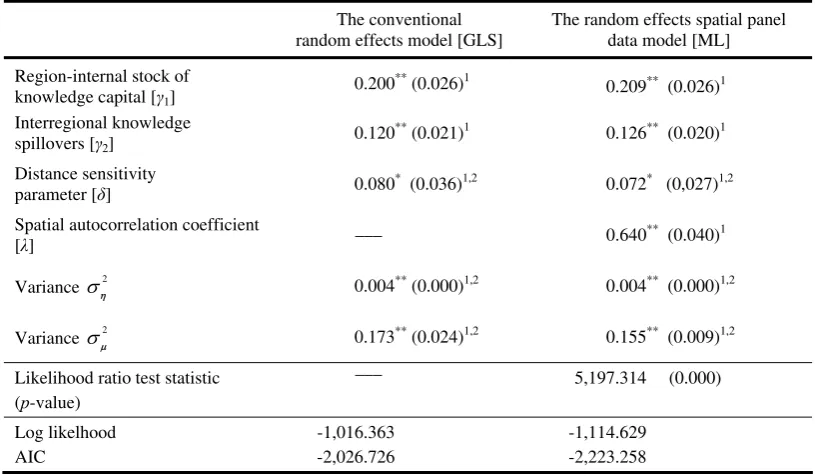
5 Estimation results
The dependent variable is region-level TFP as defined by Equation (9). The regressors are
random region effects which are assumed to be (0, 2),
iid ση the region-internal knowledge capital stock and the knowledge spillover pool variable defined as a spatially discounted sum of
the time-lagged internal knowledge stocks of all other regions as described by Equations (5)-(6).
The estimates are presented in Table 1 together with their standard errors, shown in parentheses.
The first column reports the results given by the conventional random effects panel data model
(10)-(11). The estimation method is GLS. The productivity effect from region-internal
15 Anselin (2001, pp. 325) pointed out that the computation of eigenvalues becomes instable when
N is larger than
16
knowledge is estimated as γ1=0.200, with a standard error of 0.026. The parameter estimate of
2 0.120
γ = determines the relative potency of distance-deflated cross-region knowledge spillovers. The parameter estimate of δ is equal to 0.080. This suggests that effective knowledge
from external regions is falling exponentially with bilateral distance. Productivity effects in
regions that are far away from the spilling-out region is much lower than in those located closer,
because knowledge diffusion and its productivity effects are geographically localized.
The second column presents the estimates of the random effects spatial panel data model. The λ
estimate is 0.640, with a standard error of 0.040. A likelihood ratio test for the null hypothesis of
0
λ= yields a 2 1
χ test statistic of 5,197.314. This is statistically significant and confirms the importance of a spatial autoregressive disturbance in the random effects model for measuring the
TFP impact of cross-region knowledge spillovers. The TFP effects of internal and out-of-region
stocks of knowledge are somewhat larger when spatial autocorrelation due to neighbouring
regions is taken explicitly into account. The strength of interregional knowledge spillovers is
about 4.7 percent higher than in the specification that neglects the importance of a spatial
autoregressive disturbance in the random effects model. The distance decay (or localization)
parameter δ is estimated to be 0.072, with a standard error of 0.027. This is consistent with the
hypothesis of geographic localization of interregional knowledge spillovers, and supports
Bottazzi and Peri’s (2003) findings on innovation and spillovers in European regions that a
significant positive impact of knowledge spillovers on innovative activities in neighbouring
regions appears to exist only for a distance up to 300 km.
Table 1 about here
These results provide a fairly remarkable confirmation of the role of interregional knowledge
spillovers as a statistically highly significant factor contributing to productivity differences
among the regions. The γ2-estimate implies that a one percent increase in the pool of
out-of-region knowledge capital raises the average total factor productivity in the spill-in out-of-region by
about 0.13 percent. This confirms that cross-region knowledge spillovers reinforce the impact of
17
weaker contribution of the region’s own knowledge stock. The evidence based on the distance
parameter, inherent in the construction of the pool of cross-region spillovers, indicates that the
benefits from out-of-region knowledge capital are to a substantial degree decreasing with
geographic distance. Formally integrating the spatial configuration of the data tends to slightly
increase the TFP effects with respect to both the region’s internal stock of knowledge and its
pool of knowledge spillovers, by about 4.5 percent, while decreasing the distance decay effect by
about 10 percent.
6 Closing comments
Although regional studies of economic growth and convergence have been recently in abundance, they characteristically focus on explaining output growth, as determined by the accumulation of physical capital, labour and some additional socioeconomic variables. The novelty of the new theory of economic growth essentially lies in explaining the growth of total factor productivity, which is the component of output growth not attributable to the accumulation of conventional input, such as labour and physical capital. This theory also underlines interregional economic relations that link a region’s productivity gains to economic
developments in other regions. For this reason, we have chosen to focus on the central link between productivity and cross-regional knowledge spillovers at the regional level. The issue is not so much a question whether or not such a relationship exists. Firm-level productivity studies and other factual knowledge in the field leave little doubt on this. The question, however, is whether or not econometric studies can characterize such a relationship in a satisfactory manner at the regional level of observation.
18
result is that knowledge spillovers and their productivity effects are to a substantial degree geographically localized, and this finding is consistent with the localization hypothesis, and supports, at the regional level, the cross-country findings of Keller (2002).
The final conclusion is about the research agenda for the future. All the computations described above capture only those contributions of knowledge that are measured at the aggregate regional level. Our current understanding may be improved by looking at industry-specific data and considering explicitly industry-specific knowledge capital stocks and spillovers. Another avenue for future research is to extend our framework to allow not only for geographical, but also for technological dependence between regions. This would permit us to quantify knowledge spillover effects arising from both spatial and technological proximity.
Acknowledgements. The authors gratefully acknowledge the grant no. P19025-G 11 provided by the Austrian Science Fund (FWF). They also wish to thank three anonymous referees, the editor, and James LeSage for their comments which substantially improved the paper.
References
Anselin, L. (2001): Spatial econometrics, in: B.H. Baltagi (ed.) A Companion to Theoretical Econometrics: Methods and Models. Oxford, Blackwell, pp. 310-330
Anselin, L. (1988): Spatial Econometrics: Methods and Models. Dordrecht, Kluwer
Anselin, L., Varga, A. and Acs, Z. (1997): Local geographic spillovers between university research and high technology innovations, Journal of Urban Economics 42, 422-448
Baltagi, B.H., Song, S.H. and Koh, W. (2003): Testing panel data regression models with spatial error correlation, Journal of Econometrics 117(1), 123-150
Bottazzi, L. and Peri, G. (2003): Innovation and spillovers in regions: Evidence from European patent data, European Economic Review 47, 687-710
Branstetter, L.G. (2001): Are knowledge spillovers international or intranational in scope? Microeconometric evidence from the U.S. and Japan, Journal of International Economics 53, 53-79
19
and Fischer, S. (eds.) NBER Macroeconomics Annual 1993, Vol. 8. Cambridge [MA], The MIT Press, pp.15–74
Caves, D., Christensen, L. and Diewert, W. (1982): Multilateral comparisons of output, input, and productivity using superlative index numbers, Economic Journal 92, 73-86
Coe, D.T. and Helpman, E. (1995): International R&D spillovers, European Economic Review 39(5), 859-887
Crescenzi, R., Rodríguez-Pose, A. and Storper, M. (2007): The territorial dynamics of innovation: A Europe-United States comparative analysis, Journal of Economic Geography 7, 673-709
Diewert, W.E. (1992): The measurement of productivity, Bulletin of Economic Research 44(3), 163-198 Doraszerlski, U. and Jaumandreu, J. (2008): R&D and productivity: Estimating production functions
when productivity is endogenous. Discussion Paper No. 2147, Harvard University, Cambridge [MA]
Döring, T. and Schnellenbach, J. (2006): What do we know about geographical knowledge spillovers and regional growth? Regional Studies 40(3), 375-395
Elhorst, J.P. (2005): Models for dynamic panels – An application to regional unemployment in the EU. 45th Congress of the European Regional Science Association, Amsterdam, 23-27 August, 2005 Elhorst, J.P. (2003): Specification and estimation of spatial panel data models, International Regional
Science Review 26(3), 244-268
European Commission (2001): The territorial dimension of research and development policy: Regions in the European research area, Directorate-General for Research, European Commission, February 2001
Fingleton, B. (2001) Equilibrium and economic growth: Spatial econometric models and simulations, Journal of Regional Science 41(1), 117-147
Fischer, M.M. and Reggiani, A. (2004): Spatial interaction models: From the gravity to the neural network approach, in Capello, R. and Nijkamp, P. (eds.) Urban Dynamics and Growth. Amsterdam, Elsevier, pp. 319-346
Fischer, M.M. and Varga, A. (2003): Spatial knowledge spillovers and university research: Evidence from Austria, Annals of Regional Science 37(2), 303-322
Fischer, M.M., Scherngell, T. and Jansenberger, E. (2006): The geography of knowledge spillovers between high-technology firms in Europe. Evidence from a spatial interaction modelling perspective, Geographical Analysis 38(3), 288-309
Griffith, D.A. (1988): Advanced Spatial Statistics. Dordrecht, Kluwer
Griliches, Z. (1995): R&D and productivity; Econometric results and measurement issues, in Stoneman, P. (ed.) Handbook of the Economics of Innovation and Technological Change. Cambridge [MA], Basil Blackwell, pp. 52-89
Griliches, Z. (1979): Issues in assessing the contribution of research and development to productivity growth, TheBell Journal of Economics 10(1), 92-116
20
Harrigan, J. (1997): Technology, factor supplies and international specialization: Estimating the neoclassical model, American Economic Review 87, 475-494
Jaffe, A.B. (1986): Technological opportunity and spillovers of R&D: Evidence from firms’ patents, profits, and market value, American Economic Review 76(5), 984-1001
Jaffe, A.B., Trajtenberg, M. and Henderson, R. (1993): geographic localization of knowledge spillovers as evidenced by patent citations, Quarterly Journal of Economics 108(3), 577-598
Kapoor, M., Kelejian, H.H. and Prucha, I.R. (2007): Panel data models with spatially correlated error components, Journal of Econometrics 140, 97-130
Keller, W. (2002): Geographic localization of international technology diffusion, American Economic Review 92(1), 120–142
LeSage, J.P. and Fischer, M.M. (2007): Spatial growth regressions: Model specification, estimation and interpretation, Working paper, available at SSRN: http://ssrn.com/abstract=980965
Los, B. and Verspagen, B. (2000): R&D spillovers and productivity: Evidence from U.S. manufacturing microdata, Empirical Economics 25, 127-148
Mairesse, J. and Sassenou, M. (1991): R&D and productivity: A survey of econometric studies at the firm level, NBER Working Paper 3666, NBER Working Paper Series, National Bureau of Economic Research, Cambridge [MA]
Nadiri, M.I. (1970): Some approaches to the theory and measurement of total factor productivity: A survey, Journal of Economic Literature 8(4), 1137-1177
Park, W.G. (1995): International R&D spillovers and OECD economic growth, Economic Inquiry 33(4), 571-591
Press, W.H., Teukolsky, S.A., Vetterling, W.T. and Flannery, B.P. (1992): Numerical recipes in C. Cambridge, Cambridge University Press
Robbins, C.A. (2006): The impact of gravity-weighted knowledge spillovers on productivity in manufacturing, Journal of Technology Transfer 33, 45-60
Scherer, F.M. (1993): Lagging productivity growth: Measurement, technology and shock effects, Empirica 20, 5-24
Solow, R.M. (1957): Technical progress and the aggregate production function, Review of Economics and Statistics 39, 312-320
21
Appendix
NUTS is an acronym of the French for the “nomenclature of territorial units for
statistics", which is a hierarchical system of regions used by the statistical office of the
European Community for the production of regional statistics. At the top of the
hierarchy are NUTS-0 regions (countries) below which are NUTS-1 regions and then
NUTS-2 regions. The sample is composed of 203 NUTS-2 regions located in the
pre-2004 EU member states (NUTS revision 1999, except for Finland NUTS revision
2003). We exclude the Spanish North African territories of Ceuta and Melilla, and the
French Départements d'Outre-Mer Guadeloupe, Martinique, French Guayana and
Réunion. Thus, we include the following NUTS 2 regions:
Austria: Burgenland; Niederösterreich; Wien; Kärnten; Steiermark;
Oberösterreich; Salzburg; Tirol; Vorarlberg
Belgium: Région de Bruxelles-Capitale/Brussels Hoofdstedelijk Gewest;
Prov. Antwerpen; Prov. Limburg (BE); Prov. Oost-Vlaanderen; Prov. Vlaams-Brabant; Prov. West-Vlaanderen; Prov. Brabant Wallon; Prov. Hainaut; Prov. Liége; Prov. Luxembourg (BE); Prov. Namur
Denmark: Danmark
Germany: Stuttgart; Karlsruhe; Freiburg; Tübingen; Oberbayern;
Niederbayern; Oberpfalz; Oberfranken; Mittelfranken; Unterfranken; Schwaben; Berlin; Brandenburg; Bremen; Hamburg; Darmstadt; Gießen; Kassel; Mecklenburg-Vorpommern; Braunschweig; Hannover; Lüneburg; Weser-Ems; Düsseldorf; Köln; Münster; Detmold; Arnsberg; Koblenz; Trier; Rheinhessen-Pfalz; Saarland; Chemnitz; Dresden; Leipzig; Dessau; Halle; Magdeburg; Schleswig-Holstein; Thüringen
Greece: Anatoliki Makedonia; Kentriki Makedonia; Dytiki Makedonia;
Thessalia; Ipeiros; Ionia Nisia; Dytiki Ellada; Sterea Ellada; Peloponnisos; Attiki; Voreio Aigaio; Notio Aigaio; Kriti
Finland: Itä-Suomi; Etelä-Suomi; Länsi-Suomi; Pohjois-Suomi
France: Île de France; Champagne-Ardenne; Picardie Haute-Normandie;
22
Poitou-Charentes; Aquitaine; Midi-Pyrénées; Limousin; Rhône-Alpes; Auvergne; Languedoc-Roussillon; Provence-Côte d'Azur; Corse
Ireland: Border, Midland and Western; Southern and Eastern
Italy: Piemonte; Valle d'Aosta; Liguria; Lombardia; Trentino-Alto
Adige; Veneto; Friuli-Venezia Giulia; Emilia-Romagna; Toscana; Umbria; Marche; Lazio; Abruzzo; Molise; Campania; Puglia; Basilicata; Calabria; Sicilia; Sardegna
Luxembourg: Luxembourg (Grand-Duché)
Netherlands: Groningen; Friesland; Drenthe; Overijssel; Gelderland; Flevoland;
Utrecht; Noord-Holland; Zuid-Holland; Zeeland; Noord-Brabant; Limburg (NL)
Portugal: Norte; Centro (P); Lisboa e Vale do Tejo; Alentejo; Algarve;
Açores; Madeira
Spain: Galicia; Asturias; Cantabria; Pais Vasco; Comunidad Foral de
Navar; La Rioja; Aragón; Comunidad de Madrid; Castilla y León; Castilla-la Mancha; Extremadura; Cataluña; Comunidad Valenciana; Islas Baleares; Andalucia; Región de Murcia
Sweden: Stockholm; Östra Mellansverige; Sydsverige; Norra
Mellansverige; Mellersta Norrland; Övre Norrland; Småland med Öarna; Västsverige
United Kingdom: Tees Valley & Durham; Northumberland & Wear; Cumbria;
23
Table 1 Total factor productivity estimation results (pooled data 1997-2002; N = 203, T = 6)
The conventional random effects model [GLS]
The random effects spatial panel data model [ML] Region-internal stock of
knowledge capital [γ1]
0.200** (0.026)1
0.209** (0.026)1
Interregional knowledge
spillovers [γ2] 0.120
** (0.021)1 0.126** (0.020)1
Distance sensitivity
parameter [δ] 0.080* (0.036)1,2 0.072* (0,027)1,2 Spatial autocorrelation coefficient
[λ] ––– 0.640** (0.040)1
Variance ση2 0.004** (0.000)1,2 0.004** (0.000)1,2
Variance σ2
μ 0.173
** (0.024)1,2 0.155** (0.009)1,2
Likelihood ratio test statistic (p-value)
––– 5,197.314 (0.000)
Log likelhood AIC
-1,016.363 -2,026.726
-1,114.629 -2,223.258
** denotes significance at the 0.001 level; and * significance at the 0.05 level; 1 standard errors in brackets;
2 standard errors based on jackknife estimates [they seem to be more reliable and – in any case – often much
[image:24.595.69.477.153.391.2]