Random matrix theory of the proximity effect in disordered wires

Random matrix theory of the proximity effect in disordered wires

M. Titov and H. Schomerus

Max-Planck-Institut fu¨r Physik komplexer Systeme, No¨thnitzer Strasse 38, 01187 Dresden, Germany 共Received 7 August 2002; revised manuscript received 22 October 2002; published 16 January 2003兲

We study analytically the local density of states in a disordered normal-metal wire共N兲at ballistic distance to a superconductor (S). Our calculation is based on a scattering-matrix approach, which concerns for wave-function localization in the normal metal, and extends beyond the conventional semiclassical theory based on Usadel and Eilenberger equations. We also analyze how a finite transparency of the NS interface modifies the spectral proximity effect and demonstrate that our results agree in the dirty diffusive limit with those obtained from the Usadel equation.

DOI: 10.1103/PhysRevB.67.024410 PACS number共s兲: 74.50.⫹r, 72.15.Rn, 73.20.Fz, 74.45.⫹c

I. INTRODUCTION

It is widely acknowledged that a piece of a normal metal that is in good contact with a superconductor acquires some superconducting properties. This phenomenon, named the proximity effect, has already been studied by Cooper1in the early 1960’s. Since then many theoretical and experimental investigations have been carried out.2 Much owed to the re-cent progress in the fabrication technology of nanostructures there is a revived interest to the proximity effect in the last decade.3 One remarkable evidence of this effect is the for-mation of a spectral gap in the normal metal, which strongly affects the low-temperature transport properties of the normal-metal–superconductor (NS) junctions. The key mechanism responsible for the appearance of the gap is the Andreev reflection at the NS boundary, which converts the dissipative electrical current into dissipationless supercurrent.4Similar mechanisms act in superconductor fer-romagnet junctions which have become an object of intense study recently.5,6

An effective experimental technique which allows for spatially resolved measurements of the electronic density in the nanostructures is the scanning tunnelling microscopy. It provides both a unique sub-meV energy sensitivity and an atomic spatial resolution. Several recent measurements of the local electronic density of states 共LDOS兲 in the NS junctions10,11,8,7,9 turned out to be in very good agreement with the predictions of quasiclassical theory12–17 of ‘‘non-equilibrium’’ superconductivity, based on the Usadel equa-tion for the diffusive transport18and the Eilenberger equation for the ballistic transport.19

The interplay of ballistic and diffusive transport becomes important when one studies local properties at short distance to an NS interface in a disordered system. Quasiparticles are then transferred to the interface by ballistic transport, while they explore the rest of the system diffusively. This situation is not covered by conventional quasiclassical theory. Quasi-classics also cannot account for the nonperturbative effects of wave-function localization, which only can be included by a fully phase-coherent approach. In this paper we present a theory that goes beyond the quasiclassical description and apply it to calculate the local density of states in an NS wire geometry near the interface, at zero temperature and vanish-ing magnetic field.

In our model the normal metal is shaped in the form of the

long disordered quantum wire, which supports N propagating modes at the Fermi level EF. The elastic scattering mean free path l in the wire is assumed to be much larger than the Fermi wave length ␭F, which corresponds to the weak dis-order. The superconductor is assumed to be clean and char-acterized by the bulk value ⌬ of the amplitude of the pair potential. The superconductor order parameter is assumed to be constant ⌬ in the superconductor and zero in the normal metal. This approximation is referred to in the literature as a ‘‘rigid boundary condition.’’20

We calculate the mean LDOS or, more precisely, its en-velope, at a distance x on the normal-metal side of the NS interface as shown schematically in Fig. 1. The envelope is obtained by averaging the LDOS over distances of the order of the Fermi wave length ␭F. The spatial averaging smears out the Friedel type oscillations and makes the LDOS inde-pendent on the position across the wire.

We study in detail the case that the distance x is small compared to the scattering mean free path l, so that ␭FⰆx Ⰶl, while the ratio between the superconductor coherence length ␰⫽បvF/⌬ and l remains arbitrary. The resulting mean LDOS found by averaging over disorder does not de-pend on x and is a smooth function of energy everywhere except at ␧⫽⌬ 共the energy ␧ is measured from the Fermi surface兲.

Our calculation is organized as follows. In Sec. II we derive a general relation between the one-point Green

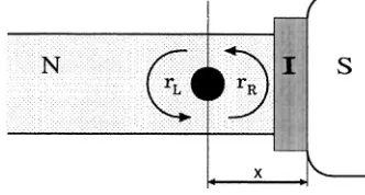
func-FIG. 1. The geometry of an NS junction consisting of a long normal-metal disordered wire N, a clean superconductor S, and a dielectric tunnel barrier I in between. The mean local density of states共LDOS兲is calculated at the distance x from the NS interface, with␭FⰆxⰆl. The matrix rLrelates the plane-wave components in the process of reflection from the normal-metal disordered wire. The matrix rR describes the reflection from the tunnel-barrier– superconductor part of the junction. The mean LDOS is found by averaging over the disorder-induced fluctuations of the matrix rL.

[image:1.612.351.517.543.632.2]

tion in a quantum wire and the reflection matrices r_L, r_R. These matrices relate the plane-wave components of the qua-siparticle wave function in the process of reflection from the parts of the wire to the left and to the right part of x.

We apply this result in Sec. III in order to calculate the mean LDOS in the neighborhood of an ideally transmitting NS interface. The matrices rL, rR of the size 2N⫻2N de-scribe the reflection of the electronlike and holelike quasipar-ticles. The left reflection matrix rL is diagonal in the electron-hole representation and depends on the disorder in the normal metal. The right reflection matrix r_R is off-diagonal共in absence of the tunnel barrier兲and is fixed within the model considered.

In the region ␧⬍⌬ we obtain the disorder-averaged LDOS

n

¯_{共x,␧兲⫽␲␳}

␧共␾A兲, ␾A⫽arccos␧/⌬, 共1兲

where the function ␳_␧(␾) is the probability density of the eigenphase of the matrix correlator r0(␧)r0(⫺␧)†. The

re-flection matrix r0(␧) relates the plane-wave amplitudes of

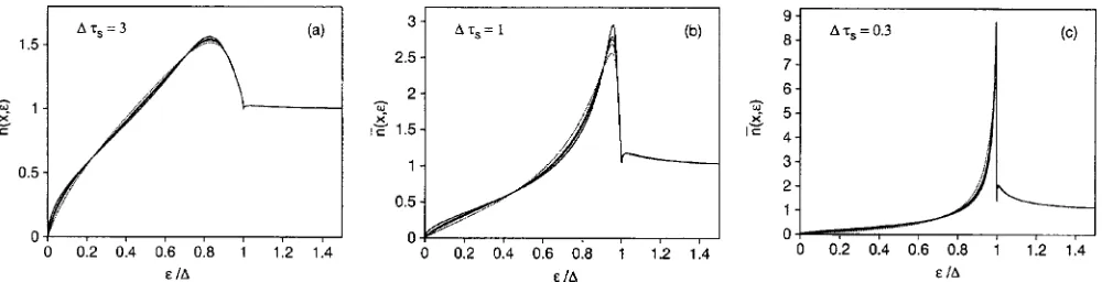
the electron wave function in the process of reflection from the semi-infinite normal-metal wire. The probability density ␳␧(␾) has been studied in Ref. 21. Apart from energy and phase it depends on the number of channels N and the mean scattering time␶s⫽l/vF. According to Ref. 21 one can dis-tinguish localized, diffusive and ballistic regimes in the form of the function␳_␧(␾) depending on the value of␧. We ob-serve the effect of Anderson localization in the linear in-crease of the LDOS for energies smaller than the Thouless energy ␧c⫽ប/N2␶s. We also find that the curves calculated for different number of channels in the wire are lying close to each other at any ratio l/␰共see Fig. 2兲. This suggests that the weak-localization correction to the LDOS is small in the case of the ideally transmitting NS interface.

In Sec. IV we generalize the model to include a tunnel barrier at the interface, parametrized by a tunnel probability per mode ⌫. We calculate analytically the LDOS near the interface in the extreme cases of a localized wire N⫽1 and a diffusive wire NⰇ1.

The effect of the tunnel barrier consists of a reduction of the pseudogap in the normal metal. This effect is most

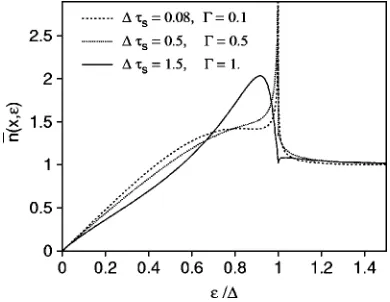
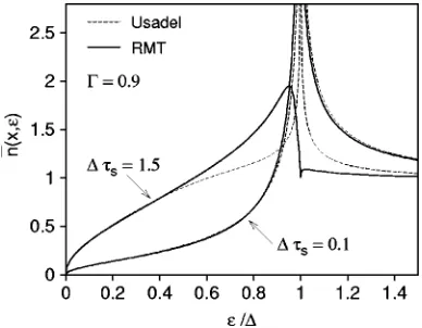
pro-nounced in the dirty regime lⱗ␰ or ⌬␶s/បⱗ1. The results of our calculation for the diffusive wire in the intermediate regime l⫽␰are summarized in Fig. 3 for different values of ⌫. We observe that the LDOS increases monotonously to its bulk constant value around the energyប⌫2/␶s and reveals a high and narrow peak close to ␧⫽⌬.

The monotonous reduction of the pseudogap is attributed to the quasiparticles which experience normal reflection at the tunnel barrier and therefore do not see the NS boundary. The formation of the peak is due to the quasiparticles re-flected from the superconductor.

When the distance x increases beyond the mean free path l a competing effect takes place. That is the suppression of the pseudogap due to the back scattering on the weak disor-der potential in the normal-metal segment of length x in front of the interface. The estimated size of the pseudogap due to this effect isបD/x2, where D is the diffusion constant in the normal metal. In this case the LDOS considerably overshoots its bulk value around␧⫽បD/x2, which is in contrast to the monotonous increase due to the tunneling into the supercon-ductor. We therefore anticipate that the effect of the tunnel barrier still can be seen in the shape of the LDOS provided បD/x2Ⰷប⌫2/␶s, or equivalently xⰆl/⌫. Namely, at

dis-FIG. 2. The mean LDOS共25兲 in an N-channel normal-metal wire near an ideally transmitting NS interface. The curves are calculated from Eqs.共24兲,共25兲. The thick solid共dotted兲line corresponds to the limiting case of the multi共single兲-channel wire. The thin lines are for the finite number of channels N⫽2, 3, and 4. The figures correspond to the clean regime⌬␶s⫽3, the intermediate regime⌬␶s⫽1, and the dirty regime⌬␶s⫽0.3.

[image:2.612.59.559.56.184.2]

tances smaller than l/⌫ the LDOS may acquire the steplike feature at the value ␧⫽ប⌫2/␶s, which is fixed by the NS interface transparency rather than by the distance to the in-terface.

A qualitatively similar phenomenon has been indeed ob-served in experiments by Levi et al.9 in the Cu barrier pin wires near a N(Cu)-S(NbTi) boundary.

On the contrary, at large distances xⰇl/⌫ the barrier is not effective in the sense that its presence cannot be distin-guished in the energy dependence of the LDOS. This is con-sistent with a general semiclassical criterion22 which states that the barrier is not effective for a given observable if the most of the relevant trajectories hit the NS interface more than⌫⫺1 times before the electron-hole coherence is lost. In the case of the LDOS this criterion is fulfilled for xⰇl/⌫.

The tunnel barrier acts differently for the single-channel wire. In the dirty regime lⱗ␰ the size of the pseudogap ប⌫/␶s scales linearly with ⌫ due to the Anderson localiza-tion. This results in a different shape of the LDOS compared to the diffusive case (NⰇ1). The difference becomes more and more pronounced with decreasing ratio l/␰ or tunneling probability⌫. In Sec. V we compare the LDOS for the dif-fusive case (NⰇ1) found from our theory to the LDOS cal-culated from the Usadel equation.14

II. GREEN FUNCTION IN A WIRE GEOMETRY

In our model of the NS junction the normal metal is shaped in the form of a semi-infinite quasi-one-dimensional disordered wire. The properties of such a system is well un-derstood in the framework of the scattering theory23provided the weak disorder limit ␭FⰆl. The detailed statistical de-scription of the disorder scattering is based on the Dorokhov-Mello-Pereyra-Kumar 共DMPK兲equation.24,25This is a scal-ing equation for the probability distribution of the scatterscal-ing matrix of a segment of the wire. Below we derive a general relation between the one-point Green function and the reflec-tion matrices rL, rR for two parts of the wire. The single-channel counterpart of this relation has been used recently to reconsider the problem of LDOS fluctuations in one-dimensional共1D兲normal-metal wires.26

The disordered wire has the Hamiltonian H⫽H0⫹V(rជ),

where V(rជ) is a disordered potential. We parametrize rជ ⫽(x,␳ជ), where x is the coordinate along the wire and␳ជ is the vector in the transversal direction. We first discuss the case of ‘‘spinless’’ electrons, assuming H0⫽⫺(1/2me)ⵜ2, ប⫽1, and include holelike quasiparticles in Secs. III and IV. In the absence of V the quantization in the transversal direction gives rise to a set of N propagating modes charac-terized by the transverse momentum qជ_n. The total energy E⫽(1/2me)(兩qជn兩2⫹kn

2

), where the x momentum kn is con-served. The retarded Green function GR(E)⫽(E⫹i␩ ⫺H)⫺1 is written in the channel representation as

G_nmR 共x,x

⬘兲

⫽

冕 冕

A

d␳ជd␳ជ

⬘

具

n兩␳ជ

典具␳

ជ

⬘

兩m

典具

rជ兩GR兩rជ

⬘

典

, 共2兲

where the integration is carried out over a cross-sectional area A. Hence the LDOS

n共rជ,␧兲⫽⫺1

␲ Im

兺

n,m

具

m兩␳ជ

典具

␳ជ兩n

典

G_nmR 共x,x兲, 共3兲

where␧ is the energy measured from the Fermi surface. For a two-dimensional wire of the width d we have

具

␳兩n

典

⫽(2/d)1/2sin(␲n␳/d). In what follows we shall omit the in-dex R, assuming everywhere the retarded Green function.

Let us formally cut the wire in the point x into two pieces and treat the left and the right part separately. We decompose the potential V⫽VR⫹VL, where VR,Lis the disorder poten-tial in the right and the left part of the wire, respectively. We also introduce the left and the right Green function as GR,L ⫽(E⫹i␩⫺H₀⫺V_L,R)⫺1_{. According to Fisher and Lee共Ref.}

27兲we have

GL,R;nm共x,x兲⫽ 1

i

冑

vnvm关␦nm⫹rL,R;nm共x兲兴, 共4兲 where vn⫽kn/me is the channel velocity and rL,R are the reflection matrices from the left and the right part of the wire, respectively.

The Green functions obey Dyson equations which can be written in the matrix form as

Gˆ共x,x兲⫽Gˆ₀共x,x兲⫹

冕

⫺⬁ ⬁

dy Gˆ₀共x, y兲Vˆ共y兲Gˆ共y ,x兲, 共5a兲

Gˆ共x,x兲⫽Gˆ_R共x,x兲⫹

冕

⫺⬁ x

d y Gˆ_R共x, y兲Vˆ_L共y兲Gˆ共y ,x兲, 共5b兲

Gˆ共x,x兲⫽GˆL共x,x兲⫹

冕

x

⬁

dy GˆL共x, y兲VˆR共y兲Gˆ共y ,x兲, 共5c兲

where the elements of the matrix Vˆ are given by

Vnm共x兲⫽

冕

A

d␳ជ

具

n兩␳ជ

典具␳

ជ兩m

典

V共rជ兲, 共6兲

and the ballistic Green function共in absence of the potential兲 reads

G0,nm共x,x

⬘兲

⫽

␦nm ivn

eikn兩x⫺x⬘兩_. 共₇兲

We also take advantage of the following relations:28

GR,nl共x, y兲⫽e⫺ikl(x⫺y )GR,nl共x,x兲 for y⬍x, 共8a兲 GL,nl共x,y兲⫽e⫺ikl(x⫺y )GL,nl共x,x兲, for y⬎x, 共8b兲 in the disorder-free regions in order to eliminate the integral terms in Eq. 共5兲. As a result we obtain the matrix equality

1 Gˆ共x,x兲⫹

1 Gˆ0共x,x兲

⫽ 1

GˆR共x,x兲

⫹ 1

GˆL共x,x兲

Using Eqs.共4兲and共7兲we finally get

Gˆ共x,x兲⫽ 1

冑

ivˆ

共1⫹rˆR兲 1

1⫺rˆLrˆR

共1⫹rˆL兲 1

冑

ivˆ

, 共10兲

where vˆ is the diagonal matrix of channel velocities vn. Together with Eq.共3兲this equation defines the LDOS via the reflection matrices. In the case of uncorrelated disorder the reflection matrices rL and rR are statistically independent, which makes Eq.共10兲useful for practical calculations.

In general the LDOS oscillates on the scale of␭F 共due to the prevailing contribution of one particular quantum state兲. These Friedel-type oscillations can play a crucial role espe-cially in one dimension. In what follows we are concerned with the smoothed version of the LDOS that does not change on the scale of the Fermi wave length and, therefore, also not in the transversal direction. For this purpose we introduce the spatially averaged LDOS

n共x,␧兲⫽␦V⫺1

冕

␦V

n共rជ,␧兲drជ, 共11兲

where the integration is carried out over a volume␦V around the point (x,␳ជ). The linear size of the volume␦V is assumed to be much larger than the Fermi wave length and much smaller than the mean free path l. For兩x⫺x

⬘

兩Ⰶl the reflec-tion matrices defined at the cross secreflec-tion x

⬘

are related to those defined at x by

r_L共x

⬘兲

⫽e⫺ikˆ(x⫺x⬘)_r

L共x兲e⫺ikˆ(x⫺x⬘), 共12a兲

rR共x

⬘

兲⫽eikˆ(x⫺x⬘)rR共x兲eikˆ(x⫺x⬘), 共12b兲

with kˆ⫽mevˆ. Expanding the right-hand side of Eq.共10兲in a geometric series in rL, rRwe notice that only the terms with equal numbers of r_Land r_R matrices do not oscillate on the scale of the Fermi wave length and have to be kept. Addi-tionally the averaging in the transversal direction mixes up the different modes so that

具

m兩␳ជ

典具

␳ជ兩n

典

⬀␦mnin Eq.共3兲. As a result we obtain

n共x,␧兲⫽n0 N Re Tr

1⫹rRrL 1⫺rRrL

, 共13兲

where n0is the bulk value of the LDOS in the normal metal,

which is set to unity in the rest of the paper. In what follows we apply Eq.共13兲to calculate the LDOS in the normal-metal wire in the immediate vicinity of an NS interface.

III. LDOS NEAR THE IDEAL NS INTERFACE

The relation共13兲applies straightforwardly to the model of the NS junction discussed in the Introduction. The only modification is the doubling of size of the reflection matrices due to particle-hole conversion. We still denote the number of electron channels in the wire by N, so that the size of the particle-hole reflection matrix is now 2N. Equation共13兲can be written in the form

n共x,␧兲⫽1⫹ 2

2N Re Trn

兺

_⫽1

⬁

共rLrR兲n, 共14兲

where rL is the electron-hole reflection matrix for the long normal-metal wire, while rR is that for the ideal NS inter-face. These reflection matrices are conveniently parametrized by

rL⫽

冉

r0共␧兲 0 0 r0共⫺␧兲*

冊

, rR⫽e⫺i␾_A

冉

0 1

1 0

冊

, 共15兲 where ␾A⫽arccos␧/⌬ is the Andreev phase and r0(␧)

⫻关r₀(␧)*_兴 is N⫻N reflection matrix of the electronlike 关holelike兴quasiparticles for the normal-metal wire. The ma-trix product rLrR is block off-diagonal, hence only the even powers n contribute to the trace in Eq. 共14兲. From Eqs. 共14兲,共15兲we obtain

n共x,␧兲⫽1⫹2

N Re Trn

兺

⫽1

⬁

关r0共␧兲r0共⫺␧兲*兴ne⫺2in␾A.

共16兲 The right-hand side of Eq.共16兲is completely determined by the eigenvalues of the correlator r0(␧)r0(⫺␧)*, which is a

unitary matrix. Its eigenvalues are conveniently parametrized by exp(2i␾j), j⫽1,2, . . . ,N, where the phases ␾j are re-stricted to the interval (0,␲). The joint probability density P_␧(␾1,␾2, . . . ,␾N) is a symmetric function with respect to

any permutation of its arguments because of the statistical equivalence of the channels. This function has been studied in detail in Ref. 21. Our calculation is restricted to the mean LDOS n¯ (x,␧)⬅

具

n(x,␧)

典

, where the angular brackets corre-spond to the average over the disorder potential in the wire. In order to perform the average in Eq.共16兲, it is enough to know only the probability density ␳_␧(␾) of a single eigen-phase. It is instructive to compare Eq.共16兲 with the similar representation of the integrated density of states in the case of the normal-metal wire of finite length, which has been analyzed recently.29

When the Andreev phase ␾A is real, i.e., for ␧⬍⌬, the mean LDOS is found from Eq.共16兲as

n

¯_{共x,␧兲⫽␲␳}

␧共␾A兲, ␧⬍⌬, 共17兲 where the eigenphase density ␳_␧(␾) is assumed to be nor-malized to unity on the interval (0,␲). The probability den-sity␳_␧(␾) acquires its simplest form in the case NⰇ1 of a large number of channels21

␳␧共␾兲⫽ 1

␲sin2_␾ Im

冑

共␧␶s兲

2_{⫹i␧␶s共1⫺e}⫺2i␾_{兲 共18兲}

and in the single-channel case30,31

␳␧共␾兲⫽␧_␲␶s

冕

0

⬁ exp共⫺␧␶st兲

transport theory ␶s

⬘

. Namely, ␶s⫽cd␶s

⬘

, where c_d ⫽2,␲2/4,8/3, for the dimensionality d⫽1,2,3, correspond-ingly.

Note, that the integrated density of states 共DOS兲 ␯ ⫽L⫺1兰₀L¯ (x,n ␧) dx in the infinite disordered wire L→⬁ is given by the relation32␯⫽␲(⳵/⳵␧)关␧␳_␧(0)兴, which is simi-lar in spirit to Eq. 共17兲. For wires with on-site disorder 共in standard universality classes兲the value of ␲␳_␧(0) equals to unity irrespective of energy␧; however it can have a singu-larity at ␧⫽0 for wires with a specific disorder symmetry.

So far we were only concerned with the mean LDOS for ␧⬍⌬. However, the result共17兲can be easily extended to the energies above the pair potential value with the help of the analytical continuation␧⫽i␻. On the other hand the analyti-cal continuation has another crucial advantage. It transforms the dynamical correlator r₀(␧)r₀(⫺␧)* into the essentially static object r0(i␻)r0(i␻)*. In the absence of a magnetic

field the time-reversal symmetry is preserved and the reflec-tion matrix r₀ is symmetric, hence r₀(i␻)*⫽r₀(i␻)†_{. The}

eigenvalues exp(2i␾j) of the matrix r0(␧)r0(⫺␧)*are

trans-formed to the real eigenvalues R_j of the matrix r0(i␻)r0(i␻)*, which are the probabilities of the reflection

from the long disordered wire in the presence of a spatially uniform fictitious absorption␻.

The summation in Eq. 共14兲 is performed in terms of the eigenvalues

n共x,␧兲⫽1 N Re

兺

j⫽1

N

1⫺Rj␣2共␻兲 1⫹Rj␣2共␻兲

冏

␻⫽⫺i␧⫹0⫹

, 共20兲

where 0⫹ is an infinitesimally small positive imaginary part of energy which ensures the retarded Green function required in Eq.共3兲. We have also introduced

␣共␻兲⫽ie⫺i␾A⫽

冑

₁⫹共␻_/⌬兲2⫺␻_/⌬_. 共₂₁兲

The joint probability density of the eigenvalues Rj for the infinitely long wire is given by the stationary solution of the DMPK equation. In the parametrization

Rj⫽ ␴j

␴j⫹2共N⫹1兲␻␶s, ␴j苸共0,⬁兲, 共22兲

this solution takes the simple form

P共兵␴j其兲⫽cN

兿

j⫽1

N

e⫺␴j/4

兿

k⬎j 兩␴k⫺␴j兩

, 共23兲

which we recognize as the orthogonal Laguerre ensemble of random matrix theory33 共with normalization constant cN). This ensemble corresponds to the class CI in the classifica-tion scheme of Ref. 34. The probability density 共one-point function兲␳(␴), normalized to unity in the interval (0,⬁), is given by35

␳共␴兲⫽e_N⫺␴

冉

兺

n_⫽0

N⫺1

关L_n(0)共␴兲兴2⫺1 2LN⫺1

(0) _共

␴兲L_N(1)_⫺1共␴兲

⫹1₄L_N(1)_⫺1共␴兲

冕

0

␴

d␨e(␴⫺␨)/2L(0)_N⫺1共␨兲

冊

, 共24兲

where L_n( p)(␴) is the generalized Laguerre polynomial. We substitute the parametrization 共22兲 in Eq. 共20兲 and average over disorder with the help of the density P(兵␴其). The result reads

n

¯_{共x,␧兲⫽Re}

冕

0

⬁

d␴ ␳共␴兲 1⫺ ␣

2_{共␻兲⫺1}

2共N⫹1兲␻␶s␴

1⫹ ␣

2_{共␻兲⫹1}

2共N⫹1兲␻␶s␴

冏

_{␻⫽⫺i␧⫹0⫹} .

共25兲 This equation extends Eq. 共17兲 to energies larger than⌬. It can also be applied for arbitrary N. In the large-N limit the distribution␳(␴) can be approximated by35

lim N_→⬁

N␳共␨N兲⫽ 1 2␲冑

4

␨⫺1, 0⬍␨⬍4. 共26兲

Substituting this expression into Eq. 共25兲 we reproduce the results of Eqs. 共17兲,共18兲 for ␧⬍⌬. In the limit ␧→0 this leads to the square root behavior of the LDOS n¯ (x,␧→0) ⫽Re

冑

⫺i␧␶s. In the extremely dirty regime⌬␶s→0 we re-produce the result of the conventional BCS theory

n

¯_{共x,␧兲⫽Re␧/}

冑

_␧2_⫺⌬2_{. 共27兲}

The Thouless energy ␧c⫽1/N2␶s, however, remains unre-solved within the multichannel approximation共26兲. In order to fix the scale ␧c one has to take advantage of another limiting relation36

lim N→⬁

␳共␨/N兲⫽J₁2共2

冑

␨兲⫺J0共2

冑

␨兲J2共2

冑

␨兲

⫹共2

冑

␨兲⫺1J0共2

冑

␨兲J1共2

冑

␨兲, 共28兲

where Jn(z) are Bessel functions. In the limit␧→0 one can safely put␣(␻)⫽1 in Eq.共25兲and take the real part explic-itly,

n

¯_{共x,␧兲⫽}

冕

0

⬁

d␴ ␳共␴兲 1

1⫹␴2关共N⫹1兲␧␶s兴⫺1. 共29兲 To leading order in␧/␧cthe function␳(␴) in Eq.共29兲can be approximated by its value at the origin ␳(0)⫽1/2, which holds for␴ⰆN⫺1 _{关see Eq. 共28兲兴. We therefore obtain}

n

¯_{共x,␧兲⫽}␲共N⫹1兲 4 ␧␶s⬇

␲

In Fig. 2 we plot the mean LDOS given by Eq. 共25兲 against the ratio␧/⌬ for different numbers of channels in the moderately dirty regime ⌬␶s⫽0.3, the intermediate regime ⌬␶s⫽1, and the moderately clean regime ⌬␶s⫽3. We ob-serve that the curves are lying close to each other in all cases. 共This suggests that the LDOS near the ideally transmitting interface is quite insensitive to phase-coherent effects.兲The situation changes in the case of a finite transparency⌫⬍1 of the NS interface.

IV. EFFECT OF A TUNNEL BARRIER

A. Model

We now introduce the simplest model of a dielectric tun-nel barrier at the ideal NS interface. The mean LDOS is calculated in the normal-metal at a ballistic distance xⰆl from the interface共see Fig. 1兲.

We describe the segment I of the wire between the chosen cross section and the ideal NS interface 共this segment in-cludes the tunnel barrier兲by its S matrix

SI⫽

冉

r₁I t₂I

t₁I r₂I

冊

, 共31兲 where each block itself consists of block-diagonal matrices in the particle-hole representation

r_1,2I ⫽

冉

r1,2共␧兲 0 0 r1,2共⫺␧兲*

冊

, 共32a兲

t_1,2I ⫽

冉

t1,2共␧兲 0

0 t1,2共⫺␧兲*

冊

, 共32b兲

and the matrices r1,2(␧), t1,2(␧) are N⫻N electron reflection

and transmission matrices corresponding to the segment I. The right matrix rR in the fundamental formula共14兲 de-pends on the S matrix of the segment I 关see Eqs.共31兲,共32兲兴 and on the scattering matrix for Andreev reflection 关see Eq. 共15兲兴. A straightforward algebraic calculation gives23

rR⫽

冉

rc共␧兲 ⫺tc共⫺␧兲* tc共␧兲 rc共⫺␧兲*

冊

, 共33a兲

tc共␧兲⫽e⫺i␾A(␧)t2共⫺␧兲*M共␧兲t1共␧兲, 共33b兲

rc共␧兲⫽r1共␧兲⫹e⫺2i␾A(␧)t2共␧兲r2共⫺␧兲*M共␧兲t1共␧兲,

共33c兲

M共␧兲⫽关1⫺e⫺2i␾A(␧)_r

2共␧兲r2共⫺␧兲*兴⫺1. 共33d兲

In general, if the segment I contains some weak disorder 共which is the case, for example, for x⬎l) the correlations between the matrices r1,2 and t1,2 for electronlike and

hole-like quasiparticles are nontrivial. We consider here the case that the segment I contains no disorder, but a sufficiently steep tunnel barrier which makes no difference in the tunnel-ing probability of electrons and holes. In this case we can omit the energy dependence in the matrices r1,2 and t1,2. In

what follows we take advantage of the polar decomposition

冉

r₁ t₂ t₁ r₂

冊

⫽

冉

uI 0 0 vI

T

冊

冉

冑

1⫺⌫ i

冑

⌫ i

冑

⌫

冑

1⫺⌫

冊

冉

u_IT 0 0 vI

冊

,

共34兲 where uI, vI are some unitary matrices, which depend on a particular realization of the barrier, and ⌫ is the diagonal matrix of the tunneling probabilities⌫j. Time-reversal sym-metry in the segment I is assumed. Once the dependence on energy in the matrices u_I,vI and⌫is disregarded we obtain from Eqs. 共33兲,共34兲the right reflection matrix

rR⫽

冉

uI 0

0 u_I*

冊

冉

ei␹ cos␪ ⫺iei␹ sin␪ ⫺iei␹ sin␪ ei␹ cos␪

冊

冉

u_IT 0 0 uI

†

冊

,

共35a兲

sin␪⫽⌫兵关1⫺e2i␾A共₁⫺⌫兲兴关₁⫺_e⫺2i␾A共₁⫺⌫兲兴其⫺1/2_,

共35b兲

e2i␹⫽共1⫺⌫⫺e2i␾A兲关₁⫺_e2i␾A共₁⫺⌫兲兴⫺1_. 共_35c兲

The left matrix rL is given by Eq. 共15兲 and describes the reflection from the disordered wire. Taking advantage of the polar decomposition we can write

rL⫽

冉

u0 0

0 u0*

冊

冉

ei␾ ₀ 0 ei␾

冊

冉

u₀T 0

0 u₀†

冊

, 共36兲 where u0 is a random unitary matrix and␾ is the diagonal

matrix of the eigenphases. We see that all information con-tained in u_I disappears statistically from the eigenvalues of rLrR because the product uI

T

u0 can be regarded again as a

random unitary matrix. Thus the disorder-averaged LDOS depends only on the transmission eigenvalues ⌫jof the tun-nel barrier. Below we calculate the mean LDOS for a single-channel wire and for a multisingle-channel wire provided the tun-neling probabilities are the same for all channels, i.e., ⌫j ⫽⌫.

B. Single channel wire

We start with the calculation of the mean LDOS for ␧ ⬍⌬ in the case of the single-channel wire N⫽1. For␧⬍⌬ the phases ␹ and␪ defined in Eq. 共35兲 are real and both r_L and rR are unitary 2⫻2 matrices. We denote uI

T u0

⫽exp(i␺), where␺ is a random phase distributed uniformly in the interval (0,2␲). We insert the reflection matrices from Eqs. 共35a兲,共36兲 directly to Eq. 共13兲. The matrix (1⫺r_Lr_R) can be easily inverted. Taking the real part we notice that the zeroes of det(1⫺rLrR) define the exact positions of the qua-siparticle bound states for␧⬍⌬. The result reads

n

¯_{共x,␧兲⫽}

冕

␪⫺␹

␲⫺␪⫺␹

d␾ ␳_␧共␾兲 sin共␾⫹␹兲

冑

cos2␪⫺cos2共␾⫹␹兲.

共38兲 In the limit ⌫→1 of the vanishing tunnel barrier one ob-serves that␹→␲/2⫺␾A and␪→␲/2, so that the area of the integration in Eq. 共37兲 shrinks to the small vicinity of ␾ ⫽␾A and the function␳_␧(␾) can be substituted by its value in this point. The integral approaches ␲ and we recover the result of Eq.共17兲for the ideally transmitting interface.

In the opposite extreme of a high tunnel barrier (⌫→0) both ␪ and␹ go to zero, so that the integration area is not restricted and the value of the integral tends to unity because of the normalization condition for the probability density ␳␧(␾). In the limit ␧Ⰶ⌬ we can set ␹⫽0 and reduce Eq. 共38兲to the following form:

n

¯_{共x,␧兲⫽Re}

冕

0

⬁

dt e⫺t

冋

1⫺ sin

2_␪

共␧␶s兲2t共t⫺2i␧␶s兲

册

⫺1/2

, 共39兲 where sin␪⫽⌫/(2⫺⌫), according to Eq.共35b兲. From Eq.共39兲 we find that

n

¯_{共x,␧兲⫽␲␧␶s}2⫺⌫

2⌫ , ␧␶sⰆ ⌫

2⫺⌫, 共40兲 which coincides for⌫⫽1 with the result of Eq. 共30兲for N ⫽1. In the dirty limit⌬Ⰶ␶s⫺1 and for a high tunnel barrier ⌫Ⰶ1 the result of Eq. 共39兲 is applicable almost up to the value of␧⫽⌬. It describes the formation of the pseudo-gap near the energy␶s⫺1⌫ due to the normal reflection from the barrier.

The exact expression 共38兲 additionally accounts for the peak at␧⯝⌬. This expression can be further generalized for energies higher than⌬ by means of the analytical continua-tion ␧⫽i␻, with the result

n

¯_{共x,␧兲⫽⫺Re}

冕

0

⬁

d␴ ␳1共␴兲

sinh Q共␴兲

冑

sinh2 Q共␴兲⫹sin2␪

, 共41a兲

Q共␴兲⫽1 2 ln

␣2_{共␻兲⫹1⫺⌫}

1⫹␣2共␻兲共1⫺⌫兲⫹ 1 2 ln

␴

␴⫹4␻␶s, 共41b兲

where the function ␳₁(␴)⫽(1/2)exp(⫺␴/2) is the probabil-ity densprobabil-ity共24兲for a single-channel wire, the function␣(␻) is defined in Eq. 共21兲, and the continuation to the real ener-gies␻→⫺i␧⫹0⫹is performed 共see Fig. 4兲.

C. Multichannel wire

The disorder-averaged LDOS for NⰇ1 can be found straightforwardly for the case of equivalent tunnelling prob-abilities ⌫j⫽⌫. Then the diagonal matrices ␪ and␹ in Eqs. 共35b兲,共35c兲 can be regarded as scalars. It is convenient to make use of the analytical continuation␧⫽i␻ and define

␣共␻兲⫽iei␾A_{, R}⫽_e2i␾_, 共_42a兲

p⫽e2i␹⫽ ␣

2_{共␻兲⫹1⫺⌫}

1⫹␣2共␻兲共1⫺⌫兲, 共42b兲 where R⫽diag(R1, . . . ,RN) is the diagonal matrix of reflec-tion probabilities for the disordered wire with a fictitious absorption␻. In the parametrization共22兲the joint probabil-ity densprobabil-ity of Rj is related to the orthogonal Laguerre en-semble 共23兲. Note that the quantities p, R_j, and␣(␻) take real values in the interval (0,1) when␻ is real.

The basic expression 共14兲 for the mean LDOS is mani-festly invariant under an arbitrary unitary rotation of the ma-trix product rLrR. From Eqs.共35a兲,共36兲we obtain

U₀†rLrRU0⫽

冉

冑

pR 0

0

冑

pR

冊

冉

cos␪ U ⫺i sin␪ ⫺i sin␪ cos␪ U†

冊

,

共43a兲

U⫽u₀TuIuI T

u0, U0⫽diag共u0,u0*兲, 共43b兲

where we take advantage of the quantities defined in Eq. 共42兲. The matrix u0 is a random unitary matrix which is

uniformly distributed in the unitary group 共provided the weak disorder kFlⰇ1). Hence by construction共43b兲, U is the unitary symmetric random matrix. We substitute Eq. 共43a兲into Eq.共14兲to express the mean LDOS as

n

¯_{共x,␧兲⫽}1 N Re Tr

冓

1⫺pR

1⫹pR

具

F共cos␪兲

典U

冔

R

, 共44兲

where

F共z兲⫽ 1

1⫺z共

冑

C1U

冑

C2⫹

冑

C2U†

冑

C1兲

, 共45a兲

C1⫽

pR

1⫹pR, C2⫽ 1

[image:7.612.340.535.58.209.2]

1⫹pR. 共45b兲 The average over disorder in Eq.共44兲is decoupled into two independent steps: the average

具•••典U

over the group

spanned by the unitary symmetric matrices and the average

具

•••典R over the orthogonal Laguerre ensemble of the reflec-tion eigenvalues Rj.

In the case of the finite number of channels the calculation of average over the unitary matrices U is technically difficult and cannot be done analytically. However, for the diffusive wire, NⰇ1, the calculation can be done by means of the diagrammatic technique developed in Ref. 37.

Let us briefly quote the basic substitution rules of the diagrammatic technique

共46兲

Here the matrix element Ui j is represented by the black and white dot connected by the dashed line. The black dot stays for the first index i and the white dot for the second index j. The conjugated matrix U* is marked by an asterisk. The other matrices are denoted by thick solid arrows. The sum-mation over a matrix index in a dot is indicated by the at-tachment of a solid line. The average over the unitary sym-metric matrices is symbolically performed by pairing in all possible ways all black and white dots belonging to U to all black and white dots belonging to U*. This pairing is de-noted by the thin solid line, which corresponds to the Kro-necker symbol. The result of the averaging is found by in-spection of the closed circuits in the diagram which consist of alternating thick and thin solid lines (T circles兲. Each diagram is weighted by a factor, which is obtained by inspec-tion of the closed circuits of alternating thin solid and dashed lines (U circles兲.

We expand the matrix F(z) 共45兲into a geometric series and keep only the terms with equal number of U and U† matrices. In the large-N limit we have to take into account the diagrams with the largest number of T circles.37 This amounts to the summation of the ‘‘rainbow’’ diagrams, or diffusion ladders, depicted symbolically in Fig. 5. The corre-sponding Dyson equation is

具

F

典

U⫽1ˆ⫹z⌺1C1

具

F

典

U⫹z⌺2C2

具

F

典

U, 共47a兲

⌺1⫽

兺

n⫽1

⬁

W_nzn⫺1关Tr C₂

具

F

典

_U兴n关Tr C₁

具

F

典

_U兴n⫺1,

共47b兲

⌺2⫽

兺

n⫽1

⬁

Wnzn⫺1关Tr C1

具

F

典

U兴n关Tr C2

具

F

典

U兴n⫺1,

共47c兲

where the weight factors

Wn⫽N1⫺2n共⫺1兲n⫺1

共2n⫺2兲!

n!共n⫺1兲!⫹O共N

⫺2n_{兲 共48兲}

have been found in Ref. 37. Taking the coefficients W_nto the leading order in N we define the generating function

h共s兲⫽

兺

n⫽1

⬁

Wnsn⫺1⫽ 1 2s共

冑

N

2_{⫹4s⫺N兲, 共49兲}

which may be used to reduce Eq.共47兲to

具

F共z兲

典

U⫽1ˆ⫹z2h共z2s1s2兲共s1C1⫹s2C2兲

具

F共z兲

典

U,

s1,2⫽Tr C1,2

具

F共z兲

典

U. 共50兲 The matrix

具

F(z)

典

_Uhas to be eliminated from the Dyson equations 共50兲. After that it is very convenient to transform to the new scalar variables

X⫽s2⫺s1

N , Y⫽

s2⫹s1

N , 共51兲

which obey the equations

X⫹1 2 ⫽

1

N Tr

1

1⫹pR f共X,Y兲, 共52a兲 Y2 sin2␪⫹X2 cos2␪⫽1, 共52b兲 with

f共X,Y兲⫽共1⫺X兲共Y⫹X兲

共1⫹X兲共Y⫺X兲, 共53兲

where we have substituted z⫽cos␪and the matrices C1, C2

from Eq. 共45b兲.

In terms of the variables X and Y the mean LDOS共44兲is simplified to

n

¯_{共x,␧兲⫽Re X}¯_{共␻兲兩␻}

→⫺i_␧⫹0⫹, 共54兲

where the bar stands for the average over the ensemble of the reflection probabilities X¯⬅

具

X

典

R.

Let us first consider the case of equal reflection probabili-ties Rj⫽R. The matrix U in Eq.共45兲commutes with C1and

C2 and can be diagonalized, hence the problem becomes

equivalent to that of a single channel wire. The solution of the self-consistent equations Eq. 共52兲is given by

X⫽⫺ sinh Q

冑

sinh2 Q⫹sin2␪, Q⫽ 1

[image:8.612.315.561.365.529.2]

2ln pR, 共55兲

which coincides with the result of the exact integration over U. This proves that the set of diagrams which we took into account in Eqs.共47兲is sufficiently complete. The substitution of Eq. 共55兲 in Eq.共54兲 and the additional average over the reflection probability of a single channel wire yields the mean LDOS of Eq. 共41兲.

In the multichannel 共diffusive兲 limit NⰇ1 the reflection probabilities R_j are, in fact, not equal. Moreover they effec-tively repel each other according to Eqs. 共22兲,共23兲. In this case Eq. 共52兲 can no longer be solved in closed form. In other words, the averages over the random matrix U and over the reflection eigenvalues R_jcannot be performed separately. In order to proceed one has to take advantage of the self-averaging property of the variables X and Y in the limit N Ⰷ1. Indeed both variables are defined via the traces s1,2and

can be thought as the arithmetic means of N fluctuating quantities. From a physical point of view the variable X is proportional to the one-point Green function, therefore it is self-averaging in a diffusive metal.

Thus we can construct the self-consistent equation for X¯ by taking the average over R on both sides of Eq.共52a兲. We assume a fixed value of f关X,Y (X)兴⫽f˜(X¯ ) on the right side, neglecting the fluctuations of X. Taking advantage of the square-root approximation 共26兲 of the density␳(␴) we ob-tain

X ¯_⫹1

2 ⫽

1 2␲

冕

0

4

d␨

冑

4 ␨⫺1

2␻␶s⫹␨

2␻␶s⫹关1⫹p f˜共X¯兲兴␨. 共56兲

The integral on the right-hand side can be carried out explic-itly giving rise to the equation

关␣2_{共␻兲⫹1⫺⌫兴关Y共X¯兲⫹X¯兴}

关1⫹␣2_{共␻兲共1⫺⌫兲兴关Y共X¯兲⫺X¯兴}

⫽1⫹ 2

1⫹X¯ 共␻␶s⫺

冑

␻␶s

冑

1⫹X

¯_{⫹␻␶s兲, 共57兲}

which is an algebraic equation for X¯ . It can be analytically continued to real energies␻⫽⫺i␧⫹0⫹and solved numeri-cally by iteration. The disorder-averaged LDOS is deter-mined, then, from Eq.共54兲. Equation共57兲is obtained in the quasiclassical limit of a large number of channels. This result does not change if we neglect that U is symmetric or take the unitary Laguerre ensemble in Eq. 共23兲 instead of the or-thogonal one.

The weak-localization correction共which we simply define as 1/N correction兲can, in principle, be determined within the present approach. It has three different sources. First of all an additional class of diagrams, namely the Cooperon-like dia-grams, have to be taken into account in the Dyson equation 共47兲. Secondly the term of subleading order in the large-N expansion of the weight factors Wn has to be included. Fi-nally the correction of order O(N⫺1) to the limiting form 共26兲 of the probability density ␳(␴) has to be considered. The calculation of the weak localization correction to the LDOS is, however, beyond the scope of this paper.

In some limiting cases Eq. 共57兲 allows for a transparent analytical solution. In the absence of the tunnel barrier ⌫ ⫽1 we obtain

X

¯_⫽1⫺2 ␣

2

1⫹␣2共1⫹⍀⫺

冑

⍀

冑

2⫹⍀兲

冏

⍀→␻␶s/(1⫹␣2)

,

共58兲 which coincides upon the substitution in Eq. 共54兲 with the result of Eq. 共25兲 in the large-N limit. In the limit ⌬␶s Ⰶ⌫2_{, Eq.共57兲leads to the BCS result for the local density,}

Eq. 共27兲.

For small energies, ␻Ⰶ⌬, we can put␣(␻)⫽1 and ob-tain

X

¯_⫽

冑

␻␶s

冑

4 sin

2_{␪⫹␻␶s⫺␻␶s}

2 sin2␪ . 共59兲

The mean LDOS共54兲for ␧Ⰶ⌬ is then given by

n

¯_{共x,␧兲⫽Re}

冑

_⫺i ␧␶s

sin2␪

冑

1⫺i ␧␶s

4 sin2␪, 共60兲 with sin␪⫽⌫/(2⫺⌫). This result describes the scaling ␧g ⬃␶s⫺1_⌫2_(2⫺⌫)⫺2 _{of the size of the pseudogap␧}

g with the transparency of the tunnel barrier ⌫, which is illustrated in Fig. 7. We observe that in the limit⌫2Ⰶ⌬␶sⰆ1 two differ-ent types of bound states contribute to the LDOS at energies below ⌬. One group of the bound states is responsible for the monotonous increase of the LDOS to its bulk value at the scale␶s⫺1⌫2 while another group gives rise to the formation of the peak near␧⫽⌬.

V. USADEL EQUATION

The aim of this section is to compare our results in the limit NⰇ1 to the results of the conventional quasiclassical theory based on the Usadel equation. It is important to re-member that the Usadel description is justified only in the dirty limit ⌬␶sⰆ1, while it is not restricted to the clean superconducting material as is the case with our calculation. In the quasiclassical context the superconductor as well as the normal metal are characterized by their diffusion con-stants Ds, Dn and normal-state resistivities␳s, ␳n, which are combined into the mismatch parameter

␥⫽_␳␳s␰s_n␰n, 共61兲

where ␰n,s⫽

冑

Dn,s/⌬ are the diffusive coherence lengths. Hence, the comparison has to be done in the limit ␥Ⰶ1, where the ‘‘rigid’’ boundary condition is valid.

⬍1), even the limit of small mismatch parameter ␥ is not completely trivial. Let us now discuss the Usadel equation for this case in somewhat more detail following the calcula-tion of Ref. 14.

The transparency of the interface enters the theory through the parameter

␥B⫽ RB

␳n␰n, 共62兲

where RB is the product of the barrier resistance and its area. The Usadel equation in the normal metal (x⬍0) takes the form

Dn

2 ⌰n

⬙共

x兲⫺␻sin⌰n共x兲⫽0, 共63兲

where ␻⫽⫺i␧⫹0⫹ is the imaginary energy, while in the superconductor (x⬎0) the equation reads

D_s

2 ⌰s

⬙共

x兲⫺␻sin⌰s共x兲⫹⌬共x兲cos⌰s共x兲⫽0, 共64兲

where⌬(x) is the gap function.共For a sake of simplicity we restrict ourselves to zero temperature.兲 The functions G(x,x)⫽cos⌰n,s(x) and F(x,x)⫽sin⌰n,s(x) parametrize normal and anomalous quasiclassical Green functions in en-ergy representation, averaged over angle and disorder. The LDOS near the interface is given by

n

¯_{共0,␧兲⫽Re cos⌰n共0兲. 共65兲}

Far away from the NS interface the Green functions aquire their bulk values

cos⌰n共⫺⬁兲⫽1, cos⌰s共⬁兲⫽ ␻

冑

⌬2_⫹␻2. 共66兲

The finite transparency of the interface comes into play in the appropriate matching conditions at x⫽012

␥B␰n⌰n

⬘共

0兲⫽sin关⌰s共0兲⫺⌰n共0兲兴, 共67a兲

␥␰n⌰n

⬘共

0兲⫽␰s⌰s

⬘共

0兲. 共67b兲 Once the superconductor is sufficiently clean the first term in Eq. 共64兲 can be disregarded, hence ⌰_s(x)⫽⌰_s(⬁) and ⌬(x)⫽⌬ for x⬎0. This justifies the ‘‘rigid’’ boundary con-ditions, which are used throughout the article.

The first integral of Eq.共63兲is readily found

D_n

4 关⌰n

⬘共

x兲兴

2_⫹␻cos⌰

n共x兲⫽const, 共68兲

where the constant is determined from the condition at x ⫽⫺⬁ and equals ␻. With the help of Eq. 共67a兲 one obtains38

sin2_关⌰

n共0兲⫺⌰s共0兲兴

4␥B2 ⫹

␻

⌬ 关cos⌰n共0兲⫺1兴⫽0, 共69兲

where ⌰_s(0) is substituted by ⌰_s(⬁) due to the ‘‘rigid’’ boundary condition. In the limit ␻Ⰶ⌬ the equation is sim-plified to

冉

cos⌰n共0兲⫺ ␻ ⌬

冊

2

⫽4␥B

2_␻

[image:10.612.156.457.57.168.2]

⌬ 关1⫺cos⌰n共0兲兴. 共70兲 Its solution gives rise to the LDOS for␧Ⰶ⌬

FIG. 6. The mean LDOS in a normal-metal wire in the vicinity of an NS interface of finite transparency. The dotted curve is found from Eq.共41兲for the single-channel wire N⫽1. The solid curve is calculated from Eqs.共54兲,共57兲for the diffusive wire NⰇ1. The dashed curve represents the result of the Usadel equation, Eqs. 共65兲,共69兲, calculated for the corresponding value of the parameter ␥B2⫽⌬␶s(2

⫺⌫)2_/(2⌫)2_{. The figures show the energy dependence of the mean LDOS for the dirty⌬␶s⫽0.3 and the clean⌬␶s⫽5 regime.}

FIG. 7. The mean LDOS in vicinity of an NS interface of finite transparency calculated from Eqs. 共54兲,共57兲. The parameters ⌬␶s and ⌫⫽0.1 are chosen to fix the combination ␥_B2⫽⌬␶s(2

[image:10.612.79.279.473.666.2]

n

¯_{共0,␧兲⫽Re}

冑

_⫺i4␧␥B

2

⌬

冑

1⫺i ␧␥B2

⌬ , 共71兲 which is manifestly equivalent to Eq.共60兲and establishes the following relation between the parameters:

␥B2_⫽⌬␶s共2⫺⌫兲 2

4⌫2 . 共72兲

This relation also follows directly from the definition of␥B, up to a numerical factor, since one can effectively substitute RB⫽(h2/e)(2⫺⌫)/2⌫, ␳n⫽(h2/e)l⫺1, and Dn⫽l2/␶s.

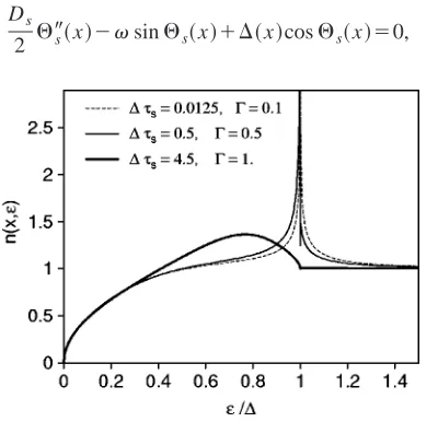
We conclude that the LDOS obtained from the Usadel equation always coincides with that found from Eq.共57兲for small energies ␧Ⰶ⌬. We also demonstrate numerically in Figs. 6, 7, and 8 that our result for NⰇ1 is perfectly consis-tent with the Usadel theory in the dirty limit⌬␶sⰆ1, where the latter is justified.

One should note, however, that the agreement with the quasiclassical theory becomes better with the increasing bar-rier height. Indeed, in the perfectly transparent interface ⌫ ⫽1, the agreement is reached only in the extremely dirty limit ⌬␶s→0, while for smaller values of ⌫ the dirty-limit condition is less restrictive关see Fig. 6共a兲兴.

VI. CONCLUSION

In conclusion, we computed the mean LDOS in a normal-metal disordered wire in the immediate vicinity of an NS

interface at zero temperature and zero magnetic field. Our calculation is based on the scattering approach and takes into account the spatial phase coherence in the normal metal.

We derived the general formula共10兲, which expresses the one-point Green function in terms of the reflection matrices. The formula can be applied in order to calculate the LDOS 共and its distribution兲 in the wire at arbitrary distance to the NS interface. In this paper we only considered the mean LDOS at the ballistic distance to the interface so that it does not acquire a spatial dependence.

We obtained the relation 共1兲 between the disorder-averaged LDOS near the ideal NS interface and the probabil-ity densprobabil-ity of the eigenphases of the matrix correlator r0(␧)r0(⫺␧)†, where r0(␧) is the reflection matrix for the

semi-infinite normal-metal wire.

We also study in detail the case of the normal-superconductor tunnel junction and derive the self-consistent equation共57兲that determines the LDOS in the diffusive nor-mal metal. In the dirty limit our expression coincides with the LDOS found by Golubov and Kupriyanov14 from the Usadel equation.

The quasiclassical analysis of the Green function at the NS interface of finite transparency has been performed by many authors12,39,14,40,41 in connection with the boundary conditions of semiclassical superconductivity. However, to our best knowledge no counterpart to Eq.共57兲 exists in the literature.

In the case of an ideal NS interface the LDOS is found to be almost independent of the number of channels in a wire, except for very small energies, hence its insensitivity to phase-coherence effects. This persists to the case of finite transparency provided the clean limit condition ⌬␶sⰇ1. In the dirty limit ⌬␶sⰆ1 and small transparency ⌫Ⰶ1/N the situation is different and the phase-coherent effects play a role.

The effect of Anderson localization is seen in the linear increase of the LDOS, n¯⫽(␲/4)(N⫹1)␧␶s(2⫺⌫)/⌫, for energies lower than ␧c⫽1/N2_{␶s. In the diffusive metal, N}

→⬁, the LDOS increases as the square root of energy n¯ ⫽Re

冑

⫺i␧␶s(2⫺⌫)/⌫. The form of the crossover in energy dependence of the LDOS from linear to square-root behavior is given by Eq.共25兲for weak disorder and perfect NS inter-face.

ACKNOWLEDGMENTS

We thank C. W. J. Beenakker, P. W. Brouwer, and R. Narayanan for helpful discussions. We are especially grateful to Alexander Golubov for bringing the results of Ref. 14 to our attention.

1_{L. N. Cooper, Phys. Rev. Lett. 6, 689共1961兲.}

2_{G. Deutscher and P. G. de Gennes, in Superconductivity, edited by} R. D. Parks共Dekker, New York, 1969兲, Vol. 2, p. 1005. 3_{Mesoscopic Electron Transport, edited by L. P. Kouwenhoven, G.}

Scho¨n, and L. L. Sohn, Vol. 345 of NATO Advanced Studies Institute, Series E: Applied Sciences共Kluwer Academic Publish-ers, Dordrecht, 1997兲.

[image:11.612.78.272.57.208.2]

4_{A. F. Andreev, Zh. E´ ksp. Teor. Fiz. 46, 1823共1964兲 关Sov. Phys.}

FIG. 8. The mean LDOS from the random matrix theory共solid lines兲, Eqs. 共54兲,共57兲, is compared to that from the Usadel theory 共dashed lines兲, Eqs.共65兲,共69兲, for the corresponding value of the parameter␥B2⫽⌬␶s(2⫺⌫2_)/(2⌫)2_{. The curves always coincide for}

JETP 19, 1228共1964兲兴.

5_{R. Fazio and C. Lucheroni, Europhys. Lett. 45, 707共1999兲; I.} Baladie´ and A. Buzdin, Phys. Rev. B 64, 224514 共2001兲; K. Halterman and O. T. Valls, ibid. 65, 014509共2001兲; F. S. Berg-eret, A. F. Volkov, and K. B. Efetov, ibid. 65, 134505共2002兲. 6_{M. A. Sillanpa¨a¨, T. T. Heikkila¨, R. K. Lindell, and P. J. Hakonen,}

Europhys. Lett. 56, 590共2001兲.

7_{S. H. Tessmer, D. J. Van Harlingen, and J. W. Lyding, Phys. Rev.} Lett. 70, 3135 共1993兲; S. H. Tessmer, M. B. Tarlie, D. J. Van Harlingen, D. L. Maslov, and P. M. Goldbart, ibid. 77, 924 共1996兲.

8_{S. Gue¨ron, H. Pothier, N. O. Birge, D. Esteve, and M. H. Devoret,} Phys. Rev. Lett. 77, 3025共1996兲.

9_{Y. Levi, O. Millo, N. D. Rizzo, D. E. Prober, and L. R.} Motow-idlo, Phys. Rev. B 58, 15 128共1998兲.

10_{N. Moussy, H. Courtois, and B. Pannetier, Europhys. Lett. 55,} 861共2001兲.

11

M. Vinet, C. Chapelier, and F. Lefloch, Phys. Rev. B 63, 165420 共2001兲.

12_{M. Yu. Kupriyanov and V. F. Lukichev, Zh. E´ ksp. Teor. Fiz. 94,} 139共1988兲 关Sov. Phys. JETP 67, 1163共1988兲兴.

13_{A. A. Golubov and M. Yu. Kupriyanov, J. Low Temp. Phys. 70,} 83共1988兲.

14_{A. A. Golubov and M. Yu. Kupriyanov, Physica C 259, 27共1996兲.} 15_{W. Belzig, C. Bruder, and G. Scho¨n, Phys. Rev. B 54, 9443}

共1996兲.

16_{S. Pilgram, W. Belzig, and C. Bruder, Physica B 280, 442共2000兲;} Phys. Rev. B 62, 12 462共2000兲.

17_{Ya. V. Fominov and M. V. Feigelman, Phys. Rev. B 63, 094518} 共2001兲.

18_{K. D. Usadel, Phys. Rev. Lett. 25, 507共1970兲.} 19_{G. Eilenberger, Z. Phys. 214, 195共1968兲.} 20_{K. K. Likharev, Rev. Mod. Phys. 51, 101共1979兲.}

21_{M. Titov and C. W. J. Beenakker, Phys. Rev. Lett. 85, 3388} 共2000兲.

22_{M. Schechter, Y. Imry, and Y. Levinson, Phys. Rev. B 64, 224513} 共2001兲.

23_{C. W. J. Beenakker, Rev. Mod. Phys. 69, 731共1997兲.}

24_{O. N. Dorokhov, Pis’ma Zh. E´ ksp. Teor. Fiz. 36, 259 共1982兲} 关JETP Lett. 36, 318共1982兲兴.

25_{P. A. Mello, P. Pereyra, and N. Kumar, Ann. Phys.共N.Y.兲181, 290} 共1988兲.

26_{H. Schomerus, M. Titov, P. W. Brouwer, and C. W. J. Beenakker,} Phys. Rev. B 65, 121101共R兲 共2002兲.

27

D. S. Fisher and P. A. Lee, Phys. Rev. B 23, 6851共1981兲. 28

V. Gasparian, T. Christen, and M. Bu¨ttiker, Phys. Rev. A 54, 4022 共1996兲.

29_{M. Titov, N. A. Mortensen, H. Schomerus, and C. W. J.} Beenak-ker, Phys. Rev. B 64, 134206共2001兲.

30_{V. L. Berezinskii and L. P. Gor’kov, Sov. Phys. JETP 50, 1209} 共1979兲.

31_{B. White, P. Sheng, Z. Q. Zhang, and G. Papanicolaou, Phys. Rev.} Lett. 59, 1918共1987兲.

32_{M. Titov, P. W. Brouwer, A. Furusaki, and C. Mudry, Phys. Rev.} B 63, 235318共2001兲.

33_{M. L. Mehta, Random Matrices共Academic, New York, 1991兲.} 34_{A. Altland and M. R. Zirnbauer, Phys. Rev. B 55, 1142共1997兲.} 35_{K. Slevin and T. Nagao, Phys. Rev. B 50, 2380共1994兲.} 36_{T. Nagao and K. Slevin, J. Math. Phys. 34, 2317共1993兲.} 37_{P. W. Brouwer and C. W. J. Beenakker, J. Math. Phys. 37, 4904}

共1996兲.

38_{The equivalent equation of Ref. 14 as well as the subsequent} discussion contain an error: the first power of␥Bappears instead of␥B

2 .

39_{A. A. Golubov and M. Yu. Kupriyanov, Zh. E´ ksp. Teor. Fiz. 96,} 1420共1989兲 关Sov. Phys. JETP 69, 805共1989兲兴.

40_{A. V. Zaitsev, Phys. Lett. A 194, 315共1994兲.}