Gesture Spotting Using Wrist Worn Microphone and 3 Axis Accelerometer

Gesture Spotting Using Wrist Worn Microphone

and 3-Axis Accelerometer

Jamie A. Ward

, Paul Lukowicz

, Gerhard Tr¨

oster

Abstract. We perform continuous activity recognition us-ing only two wrist-worn sensors - a 3-axis accelerometer and a microphone. We build on the intuitive notion that two very different sensors are unlikely to agree in classification of a false activity. By comparing imperfect, sliding window classi-fications from each of these sensors, we are able discern ac-tivities of interest from null or uninteresting acac-tivities. Where one sensor alone is unable to perform such partitioning, using comparison we are able to report good overall system perfor-mance of up to 70% accuracy. In presenting these results, we attempt to give a more-in depth visualization of the errors than can be gathered from confusion matrices alone.

1

Introduction

Hand actions play a crucial role in most human activities. As a consequences detecting and recognising such activities is one of the most important aspects of context recognition. At the same it is one of the most difficult. This is particularly true for continuous recognition where a set of relevant hand motions (gestures) need to be spotted in a data stream. The difficulties of such recognition stem from two things. First, due to a large number of degrees of freedom, hand motions tend to be very diverse. The same activity might be performed in many different ways even by a single person. Second, in terms of motion, hands are the most active body parts. We move our hands continuously, mostly in an unstructured way, even when not doing anything particular with them. In fact in most situations such unstructured motions by far outnumber gestures that are relevant for context recognition. This means that a continuous gesture spotting applications has to deal with an zero class that is difficult to model while taking up most of the signal.

1.1

Paper Contributions

Our group has invested a considerable amount of work into hand gesture spotting. To date this work has focused on using several sensors distributed over the user’s body to maximise system performance. This included motion sensors (3 axis ac-celerometer, 3 axis gyroscopes and 3 axis magnetic sensors) on the upper and lower arm [3], microphone/accelerometer combination on the upper and lower arm [5] as well as, more

1

Swiss Federal Institute of Technology (ETH), Wearable Comput-ing Lab, Zurich

2

UMIT (University of Health Sciences, Medical Informatics and Technology, Hall i. Tirol, Austria

3

ETH, Wearable Computing Lab, Zurich

recently, a combination of several motion sensors and ultra-sonic location devices.

This paper investigates the performance of a gesture spot-ting system based on a single, wrist mounted device. The idea behind the work is that wrist mounted accessories are broadly accepted and worn by most people on daily basis. In contrast, systems that require the user to put on several sensors at loca-tions such as the upper arm would have much more problems with user acceptance.

The downside of this approach is the reduced amount of information available for the recognition. This for example means that the method of analysing sound intensity differ-ences between microphones on different parts of the body that was the corner stone of our previous signal partitioning work is not feasible. This problem is compounded by the fact that for the approach to make sense that wrist mounted device can neither contain too many sensors nor can it require computing and/or communication power that would imply large, bulky batteries.

The main contribution of the paper is to show that, for a certain subset of activities, reasonable gesture spotting results can be achieved with a combination of a microphone and 3 axis accelerometer mounted on the wrist. Our method relies on simple jumping window sound processing algorithms that we have shown [10] to require only minimal computational and communication performance. For the acceleration we use inference on Hidden Markov Models (HMM), again on jump-ing windows across the data.

To our knowledge this is the first time that such a simple system and a straight forward jumping window method has been successfully used for hand gesture spotting in contin-uous data stream with a dominant, unstructured zero class. Previously such setups and algorithms have only been shown to be successfull either for segmented recognition or for sce-narios where the zero class was either easy to model or not relevant (e.g. recognition of standing, sitting, walking, run-ning [6, 9, 12]). Where these approaches use acceleration sen-sors, in the work of [?,?] sound was exploited for performing situation analysis in the wearable computing domain. Also

[?] used sound information to improve the performance of

hearing aids. Complimentary information from sound and ac-celeration has been used before to detect defects in material surfaces, e.g. in [13], but no work that the authors are aware uses these for recognition of complex activities.

to achieving good performance despite simple sensors and algorithms. We verify our approach on data from a wood workshop assembly experiment that have we have introduced and used in previous work [5]. We present the results using both traditional confusion matrices, plus a novel visualisation method that provides a more in-depth understanding of the error types.

2

Recognition Method

We apply sliding windows of lenght wlen seconds across all

the data in increments of wjmp. At each step we apply an

LDA based classification on the sound data, and an HMM classification on the sound. The ’soft’ results of each classifi-cation - LDA distances for sound and HMM class likelihoods for acceleration - are converted into class rankings, and these are fused together using one of two methods: comparison of top rank (COMP), and a method using Logistic Regression (LR).

2.1

Frame by Frame Sound Classification

Using LDA

Frame-by-frame sound classification was carried out using pattern matching of features extracted in the frequency do-main. Each frame represents a window on 100ms of raw audio data. These windows are then jumped over the entire dataset in 25ms increments, producing a 40Hz output.

The audio stream was taken at a sample rate of 2kHz from the wrist worn microphone. From this a Fast Fourier Trans-form (FFT) was carried out on each 100ms window, generat-ing a 100 bin output vector (1/2∗f s∗f f twnd= 1/2∗2∗100 = 100bins).

Making use of the fact that our recognition problem re-quires a small finite number of classes, we applied Linear Dis-criminant Analysis (LDA)[1] to reduce the dimensionality of

these FFT vectors from 100 to #Classes−1.

Classification of each frame can then be carried out using a simple Euclidean minimum distance calculation. Whenever we wish to make a decision, we simply calculate the incoming point in LDA space and find its nearest class mean value from the training dataset. This saving in computation complexity by dimensionality reduction comes at the comparatively mi-nor cost of requiring us to compute and store a set of LDA class mean values from which the LDA distances might be obtained.

Equally, a nearest neighbour approach might be used. For the experiment described here however, Euclidean distance was found to be sufficient.

A larger window, wlen, was moved over the data inwjmp

second increments. This relatively large window was chosen to reflect the fact that all of the activities we are interested in occur at the timescale of at least several seconds. On each win-dow we compute a sum of the constituent LDA distances for each class. From these total distances, we then rank each class according to minimum distance. Classification of the window is then simply a matter of choosing the top ranking class.

2.2

HMM Acceleration Classification

In contrast to the approach used for sound recognition, we employed model based classification, specifically the Hidden

Markov Model (HMM), for classifying accelerometer data[8, 11]. (The implementation of the HMM learning and inference routines for this experiment was provided courtesy of Kevin P. Murphy’s HMM Toolbox for matlab [7].)

The features used to feed the HMM models were calculated from sliding 100ms windows on the x,y, and z axis of the 100Hz sampled acceleration data. These windows were moved over the data in 25ms increments, producing the following features, output at 40Hz:

• Mean of x-axis

• Variance of x-axis

• A count of the number of peaks (for x,y,z)

• Mean amplitude of the peaks (for x,y,z)

Finally we globally standardised the features so as to avoid numerical complications with the model learning algorithms in matlab.

In previous work we employed single Gaussian observation models, but this was found to be inadequate for some classes unless a large number of states were used. Intuitively, the descriptive power of a mixture of Gaussian is much closer to ’reality’ than only one, and so for these classes a mixture model was used. The specific number of mixtures and the number of hidden states used were individually tailored by hand for each class. The parameters themselves were trained from the data.

A window of wlen, in wjmp increments, was run over the

acceleration features, and the corresponding log likelihood for each HMM class model calculated.

Classification is carried out for each window by choosing the class which produces the largest log likelihood given the stream of feature data from the test set.

2.3

Fusion of classifiers

Comparison of top choices (COMP) The top rankings

from each of the sound and acceleration classifiers for a given jumping window segment are taken, compared, and returned as valid if they agree. Those where both classifiers disagree are thrown out - classified as null.

Logistic regression (LR) The main problem with a di-rect comparison of top classifier rankings is that it fails to take into account cases where one classifier might be more reliable than another at recognising particular classes. If one classifier reliably detects a class, but the other classifier fails to, perhaps relegating the class to second or third rank, then a basic comparison would just assign null. For such cases, then a ’softer’ method of classifier fusion is needed - one that takes into account the different rankings of each classifier.

In the work of Ho et. al. [2], three methods for classifier fusion based on class rankings are presented and evaluated: Highest Rank, whereby each class is assigned a rank according to the highest rank assigned to it by any of the classifiers; Borda count, whereby each class is ranked according to the total number of classes ranking below it by each classifier; and Logistic Regression (LR), a method based on the Borda count, but which estimates weights for each class combination using regression.

one which provides the scope to deal with assigning results to null.

The basic motivation behind LR is to assign a score for each class and every combination of classifier rankings. How-ever, such a scoring would soon become computationally pro-hibitive, even for a moderate number of classes and classifiers. Instead, LR makes use of a linear function to estimate the likelihood of whether a class is correct or not for a given set of rankings. Such a regression function, estimating a binary outcome with P(true|X, class) or P(f alse|X, class), would be far simpler to compute. So for each class a function can be computed: L(X) =α+Pm_i=1βixi where X = [x1, x2, ..xm]

are the rankings of the class for each of the m classifiers, and

α,βthe logistic regression coefficients. These coefficients can be computed by applying a suitable regression fit using the correctly classified ranking combinations from, for example, training data.

So that unlikely combinations are assigned to null, we intro-duce an empirically obtained threshold onL(x) for each class. Of the classes which fall below this threshold, the most likely

L(x) value is taken and re-assigned to the ’null class’. This means that if all classes fall below their threshold for a given ranking combination, then the null will take top ranking.

Classification can then be carried out by estimating L(X) for each class on the input rankings, comparing with the null threshold, and then ranking the values obtained. The final classification result can then be taken from the highest rank.

3

Experimental setup

Data was collected using a sony microphone and a 3-axis accelerometer (from the ETH PadNET sensor network [4]) strapped to the wrist. Each subject was asked to follow a pre-defined sequence of activities using tools in the wood work-shop of our lab. The 9 activities which we set out to spot were: hammering (h), sawing (s), filing (f), using a machine drill (r), sanding (a), using a machine grinder (g), screwdriv-ing (w), openscrewdriv-ing and closscrewdriv-ing a vise (v), openscrewdriv-ing and closscrewdriv-ing a drawer (d). All other activities and movements were labelled as null (φ).

Each subject performed the entire sequence in about 5 min-utes. In all, twenty such sets of data were collected from five different subjects.

4

Results

The system was initially evaluated across sweeps of the two

main parameters, window length wlen and window jump

lenghtwjmp. From these sweeps, setting bothwlenandwjmp

to 2 seconds was found to produce favourable results. All fur-ther analysis was carried out with these parameters set.

Both the LDA and HMM methods require training of pa-rameter using data. This was carried out in a user-dependent leave-one-out fashion. That is for each set under test, the training data was taken from the sets of the same user but not including the set under test.

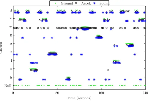
We applied HMM classification to the accelerometer data, and LDA minimum distance to the audio. This was applied to all 20 sets of data. Typical results from one of these sets is plotted in Figures 1, with class predictions compared along-side the hand-labelled ground truth.

With each of the 2 second segments, we then carried out firstly the classification comparison fusion, and then the lo-gistic regression using the rankings obtained from the HMM likelihood and LDA distance information.

On first run, the LR method continued to produce a large number of insertions - primarily from the class ’screwdriving’. This was due to the fact that this is comparatively silent class, and as the training data consisted mostly of noisy, positive class examples (at no stage do we use null labelled data for training), it winds up being a ’catch all’ class for non-activities which should have been assigned null. Reducing the weights of the ranking combinations for this class during training helps to alleviate this problem.

The final predictions from each of these, compared along-side the ground truth, are shown in 2.

PSfrag replacements

Time (seconds)

Classes

Sound

Ground Accel. Sound

0 80 160 240

320 400 480 560 640 720 800 880 960 1040 1120 1200 1280 1360 1440 1520 1600 1680 1760 1840 1920 2000 2080 2160 2240 2320 2400 2480 2560 2640 2720 2800 2880 2960 3040 3120 3200 3280 3360 3440 3520 3600 3680 3760 3840 3920 4000 4080 4160 4240 4320 4400 4480 4560 4640 4720 4800 4880 4960 5040 5120 5200 5280 5360 5440 5520 5600 5680 5760 5840 5920 6000 6080 6160 6240 6320 6400 6480 6560 6640 6720 6800 6880 6960 7040 7120 7200 7280 7360 7440 7520 7600 7680 7760 7840 7920 8000 8080 8160 8240 8320 8400 8480 8560 8640 8720 8800 8880 8960 9040 9120 9200 9280 9360 9440 9520 9600 9680 9760 9840 9920 10000 10080 10160 10240 10320 10400 10480 10560 10640 10720 10800 10880 10960 11040 11120 11200 11280 11360 11440 11520 11600 11680 11760 11840 11920 12000 Null h s f r a g w v d

Figure 1. Plot of a typical output sequence - shown is the

ground truth, the Sound predictions and acceleration predictions.

PSfrag replacements

Time (seconds)

Classes

LR

Ground Comb. LR

0 80 160 240 320 400 480 560 640

720 800 880 960 1040 1120 1200 1280 1360 1440 1520 1600 1680 1760 1840 1920 2000 2080 2160 2240 2320 2400 2480 2560 2640 2720 2800 2880 2960 3040 3120 3200 3280 3360 3440 3520 3600 3680 3760 3840 3920 4000 4080 4160 4240 4320 4400 4480 4560 4640 4720 4800 4880 4960 5040 5120 5200 5280 5360 5440 5520 5600 5680 5760 5840 5920 6000 6080 6160 6240 6320 6400 6480 6560 6640 6720 6800 6880 6960 7040 7120 7200 7280 7360 7440 7520 7600 7680 7760 7840 7920 8000 8080 8160 8240 8320 8400 8480 8560 8640 8720 8800 8880 8960 9040 9120 9200 9280 9360 9440 9520 9600 9680 9760 9840 9920 10000 10080 10160 10240 10320 10400 10480 10560 10640 10720 10800 10880 10960 11040 11120 11200 11280 11360 11440 11520 11600 11680 11760 11840 11920 12000 12080 Null h s f r a g w v d

Figure 2. Plot of output sequence of sound and acceleration

predictions combined, versus ground truth.

the constituent classifiers, as expected, produce much noise. With LDA tending to misclassify null as a quiet class, such as screwdriving; and HMM generally giving random misclassifi-cations. Both perform relatively well when set against known system classes however, and this is reflected in the perfor-mance of both the comparison and LR predictions.

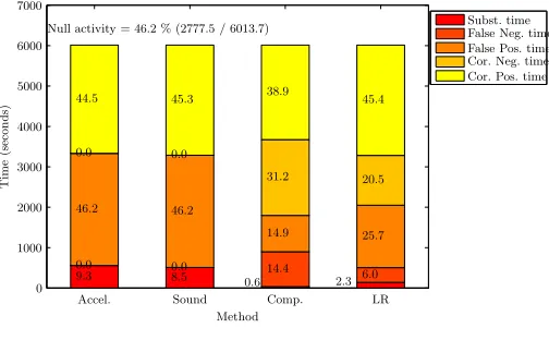
Plotting predictions might allow us to gain a rough under-standing of how well the system performs for a given set, but for a measure across all the data we require a more quanti-tative means. For this we perform a direct frame by frame comparison of the predictions with the ground truth, and fill out a confusion matrix of the results. We sum the matrices across all test datasets and present the total matrix, for each recognition method, in Tables 1. Class by class recognition rates, stating how well the system returns true frames are given to the right of these tables. Also shown is a summary of the False Positive (FP), False negative (FN), Substitution, Correct True Positive (cTP) and the overall Accuracy as per-centages of the total experiment time.

By way of summary of these tables we also show the substi-tution false negative, false positive and the correct negative, correct positive times as a percentage of the entire dataset in the barcharts of Figure 3.

PSfrag replacements

Method

Time

(seconds)

9.3 0.0 46.2 0.0 44.5

8.5 0.0 46.2 0.0 45.3

0.6 14.4 14.9 31.2 38.9

2.3 6.0 25.7 20.5 45.4

Null activity = 46.2 % (2777.5 / 6013.7) Subst. time_{False Neg. time}

False Pos. time Cor. Neg. time Cor. Pos. time 0

0.1 0.2 0.3 0.4 0.5 0.6 0.7 0.8 0.9 1

Accel. Sound Comp. LR

0 0.1 0.2 0.3 0.4 0.5 0.6 0.7 0.8 0.9 1

0 1000 2000 3000 4000 5000 6000 7000

Figure 3. Breakdown of errors as a percentage of total

experiment time for acceleration, sound and combined: Correct Positive, Correct Negative, False Positive, False Negative and Substitution times, as taken directly from the confusion matrix

Continuous recognition systems which deal with human ac-tivity are often characterised by the lack of fixed, well-defined activity boundaries. In many cases, whether an activity was recognised exactly within the labelled time frame, or slightly off from it, is less important than the fact that the activity was detected correctly in the first place. The confusion matrix based evaluation as given does not account for such ’fuzzy’ boundaries, and makes a strict judgement on the predicted frames according to the given ground truth.

If we lighten this restriction, we can create two additional error classifications, which we calloverf illandunderf ill, as defined:

• Overfill time: when a continuous sequence of correct predic-tion frames slips over the ground truth boundary to cover null labelled frames (previously classed as insertion time)

• Underfill time: the time left when a continuous sequence

of correct prediction frames does not completely cover the corresponding ground truth (previously classed as deletion time)

Taking account of this, the total overfill and underfill, to-gether with substitution, deletion, insertion, correct positive and correct negatives times as a percentage of the overall ex-periment, are shown in Figure 4. To mark the level of true insertion, deletion and substitution errors, we introduce a ’se-rious error’ measure, as shown on the charts.

PSfrag replacements

Method

Time

(seconds)

9.3 0.0 10.2

19.5% 0.0 36.0 0.0 44.5

8.5 0.0 16.7

25.1% 0.0 29.5 0.0 45.3

0.6 3.9 2.8 7.2%

10.5 12.2 31.2 38.9

2.35.4 1.6 9.4% 4.4 20.3 20.5 45.4

Null activity = 46.2 % (2777.5 / 6013.7) Subst. time_{Del. time}

Ins. time Underfill time Overfill time Cor. Neg. time Cor. Pos. time 0

0.1 0.2 0.3 0.4 0.5 0.6 0.7 0.8 0.9 1

Accel. Sound Comp. LR

0 0.1 0.2 0.3 0.4 0.5 0.6 0.7 0.8 0.9 1

0 1000 2000 3000 4000 5000 6000 7000

Figure 4. Breakdown of errors as a percentage of total

experiment time for acceleration, sound and combined: Correct Positive, Correct Negative, Overfill, Underfill, Insertion, Deletion

and Substitution times; also given is the ’serious error’ level, which ignores the minor errors of Overfill and Underfill

5

Discusion

As expected, the individual recognition performance for each of the two sensor types performed quite poorly on their own, but once combined the results improved dramatically.

As a percentage of the entire time, substitution of one pos-itive class for another decreased from a maximum of 9.3% by HMM on acceleration to as low as 0.6% in the comparison fusion (and a respectable 2.3% for LR).

The amount of false positives as a percentage of total time fell to 14.9% for comparison. LR, which although fairs less well at 25.7% FP, is however the better choice for fewer false negatives (6% compared to comparison’s 14.4%).

When underfill and overfill are considered, these results be-gin to take on new meaning, as the more serious errors of insertions and deletions prove to occur far less than the count of FP and FN might suggest. As a percentage of the total time, the sum of insertion, deletion and substitution errors is only around 7% for COMP and 9% for LR.

5.1

Conclusion

Gnd(T) h s f r a g w v d φ %Correct

h( 195.7) 183.6 2.5 3.6 0.6 2.4 3.0 93.84

s( 306.4) 3.7 209.9 69.7 3.9 4.0 15.2 0.1 68.50 f( 304.6) 0.6 40.3 248.3 1.9 8.0 0.3 4.9 0.2 81.52

r( 241.5) 0.9 184.0 50.6 2.0 4.0 76.20

a( 313.0) 0.7 3.3 40.5 6.3 228.2 2.7 29.6 1.8 72.91

g( 277.7) 15.1 260.6 2.0 93.85

w( 260.4) 19.3 2.0 2.0 229.7 7.3 88.23

v( 678.1) 65.2 28.5 0.4 11.4 4.6 543.4 24.6 80.14

d( 658.8) 8.2 30.3 10.9 7.4 12.0 590.1 89.57

φ(2777.5) 185.9 12.5 13.5 471.5 1.8 304.9 77.2 296.3 1413.9 0

Accel. Total: 6013.7 FN: 0.0 FP: 2777.5 Subst.: 558.2 cTP: 2678.0 cTP+TN: 2678.0 0.0% 46.2% 9.3% 44.5% Accuracy: 44.5%

Gnd(T) h s f r a g w v d φ %Correct

h( 195.7) 168.5 19.6 6.7 0.8 86.12

s( 306.4) 267.2 14.0 2.0 10.5 12.7 87.21

f( 304.6) 238.8 34.4 1 16.1 2.5 2.8 78.40

r( 241.5) 226.5 12.0 2.0 1.0 93.79

a( 313.0) 6.0 13.9 258.0 2.0 21.7 0.9 10.5 82.42

g( 277.7) 2.9 274.5 0.3 98.86

w( 260.4) 249.0 9.8 1.6 95.64

v( 678.1) 0.3 101.8 571.2 4.8 84.24

d( 658.8) 0.7 163.6 22.7 471.8 71.61

φ(2777.5) 5.5 8.8 7.3 111.5 18.0 67.5 1360.8 506.4 691.7 0

Sound Total: 6013.7 FN: 0.0 FP: 2777.5 Subst.: 510.6 cTP: 2725.6 cTP+TN: 2725.6 0.0% 46.2% 8.5% 45.3% Accuracy: 45.3%

Gnd(T) h s f r a g w v d φ %Correct

h( 195.7) 168.5 0.6 1.3 0.8 24.5 86.12

s( 306.4) 200.3 12.0 5.0 89.1 65.38

f( 304.6) 203.3 2.0 0.3 99.1 66.73

r( 241.5) 169.0 72.5 69.99

a( 313.0) 194.6 1.1 0.9 116.4 62.16

g( 277.7) 259.5 18.2 93.45

w( 260.4) 225.7 34.6 86.70

v( 678.1) 1.7 476.2 1.0 199.2 70.23

d( 658.8) 5.4 2.1 44 211.3 66.79

φ(2777.5) 3.5 1.7 2.7 83.0 1.4 50.5 67.2 126.1 562.2 1879.2 67.66

Comp. Total: 6013.7 FN: 864.9 FP: 898.3 Subst.: 34.1 cTP: 2337.1 cTP+TN: 4216.4 14.4% 14.9% 0.6% 38.9% Accuracy: 70.1%

Gnd(T) h s f r a g w v d φ %Correct

h( 195.7) 169.5 0.6 4.1 2.2 19.4 86.61

s( 306.4) 254.3 22.0 9.4 0.1 20.6 83.00

f( 304.6) 4.0 262.2 12.0 0.3 3.1 0.2 22.9 86.07

r( 241.5) 232.3 4.2 5.0 96.19

a( 313.0) 8.0 22.8 237.6 1.1 8.8 1.1 33.7 75.89

g( 277.7) 275.6 2.1 99.26

w( 260.4) 225.7 2.8 31.8 86.70

v( 678.1) 0.3 1.7 566.7 17.7 91.7 83.58

d( 658.8) 5.4 8.1 508.5 136.8 77.19

φ(2777.5) 10.5 9.7 7.1 121.7 2.4 76.2 67.2 282.8 969.4 1230.6 44.30

LR Total: 6013.7 FN: 363.8 FP: 1546.9 Subst.: 139.9 cTP: 2732.5 cTP+TN: 3963.1 6.0% 25.7% 2.3% 45.4% Accuracy: 65.9%

Table 1. Confusion matrices for the acceleration, sound, comparison (Comp.) and logistic regression (LR) classifications with sliding

window of 2 seconds. The total % Correct is a summation of the class correct times over the total time. All times are given in seconds.φ

denotes the ’Null’ class.

using standard sliding window based approaches. Alone, nei-ther sensor can detect a null gesture, but when fused togenei-ther, this becomes possible. Achieving, in this experiment, overall accuracies of around 70% for classifier result comparision and 66% for a method using logistic regression (LR). We also in-troduce the terms ’underfill’ and ’overfill’ to describe those common cases in continuous recognition where events fail to completely match the ground truth - but which might actu-ally be judged correct by a human observer - and show how these can be applied in visualizing results.

6

Acknowledgements

The authors would like to thank Thad Starner from Georgia Institute of Technology for his invaluable advice and support in this work.

References

[1] R. Duda, P. Hart, and D. Stork. Pattern Classification, Sec-ond Edition. Wiley, 2001.

[2] Tin Kam Ho, J.J. Hull, and S.N Srihari. Decision combination in multiple classifier systems. volume 16, pages 66–75, Jan 1994.

[3] Holger Junker, Paul Lukowicz, and Gerhard Tr¨oster. Con-tinuous recognition of arm activities with body-worn inertial sensors. InISWC, pages 188–189, 2004.

[4] N. Kern, B. Schiele, H. Junker, P. Lukowicz, and G. Tr¨oster. Wearable sensing to annotate meeting recordings. InIEEE Int’l Symp. on Wearable Computers, pages 186–193, October 2002.

[5] Paul Lukowicz, Jamie A Ward, Holger Junker, Gerhard Tr/oster, Amin Atrash, and Thad Starner. Recognizing work-shop activity using body worn microphones and accelerome-ters. InPervasive Computing, 2004.

[6] J. Mantyjarvi, J. Himberg, and T. Seppanen. Recognizing human motion with multiple acceleration sensors. In 2001 IEEE Int’l Conf. on Systems, Man and Cybernetics, volume 3494, pages 747–752, 2001.

[7] Kevin P. Murphy. The hmm toolbox

for MATLAB, http://www.ai.mit.edu/

mur-phyk/software/hmm/hmm.html.

[8] L. R. Rabiner and B. H. Juang. An introduction to hidden Markov models.IEEE ASSP Magazine, pages 4–16, January 1986.

[9] C. Randell and H. Muller. Context awareness by analysing accelerometer data. InIEEE Int’l Symp. on Wearable Com-puters, pages 175–176, 2000.

[10] Mathias St¨ager, Paul Lukowicz, Gerhard Tr¨oster, and Thad Starner. Implementation and evaluation of a low-power sound-based user activity recognition system. 8th Int’l Symp. on Wearable Comp., 2004.

[11] T. Starner, J. Makhoul, R. Schwartz, and G. Chou. On-line cursive handwriting recognition using speech recognition methods. InICASSP, pages 125–128, 1994.

[12] K. Van-Laerhoven and O. Cakmakci. What shall we teach our pants? InIEEE Int’l Symp. on Wearable Computers, pages 77–83, 2000.