Interaction rates in string gas cosmology
Rebecca Danos*Department of Physics, University of California, Los Angeles, Los Angeles, California 90095, USA Andrew R. Frey†
California Institute of Technology, 452-48, Pasadena, California 91125, USA Anupam Mazumdar‡
NORDITA, Blegdamsvej-17, DK-2100, Copenhagen, Denmark (Received 1 October 2004; published 29 November 2004)
We study string interaction rates in the Brandenberger-Vafa scenario, the very early universe cosmology of a gas of strings. This cosmology starts with the assumption that all spatial dimensions are compact and initially have string scale radii; some dimensions grow due to some thermal or quantum fluctuation which acts as an initial expansion velocity. Based on simple arguments from the low-energy equations of motion and string thermodynamics, we demonstrate that the interaction rates of strings are negligible, so the common assumption of thermal equilibrium cannot apply. We also present a new analysis of the cosmological evolution of strings on compact manifolds of large radius. Then we discuss modifications that should be considered to the usual Brandenberger-Vafa scenario. To confirm our simple arguments, we give a numerical calculation of the annihilation rate of winding strings. In calculating the rate, we also show that the quantum mechanics of strings in small spaces is important.
DOI: 10.1103/PhysRevD.70.106010 PACS numbers: 11.25.Wx, 98.80.Cq
I. INTRODUCTION
In [1], Brandenberger and Vafa (BV) proposed a seem-ingly very natural initial condition for cosmology in string theory. In BV cosmology, all nine spatial dimen-sions are compact (and toroidal in the simplest case) and initially at the string radius. The matter content of the universe is provided by a Hagedorn temperature gas of strings. In addition to proposing a very interesting initial condition and analyzing the thermodynamics of strings at that point, however, BV argued that string theory in such a background provides a natural mechanism for decom-pactifying up to three spatial dimensions (that is, allow-ing three spatial dimensions to become macroscopic). The BV mechanism works because winding strings provide a negative pressure, which causes contraction of the scale factor, as was shown explicitly in [2,3]. BV then gives a classical argument that long winding strings can cross each other only in three or fewer large spatial dimensions. Therefore, since winding strings freeze out quickly in four or more large spatial dimensions, the winding strings would cause recollapse of those large dimensions.
Reference [1] has inspired a broad literature. One im-portant generalization has been including branes in the early universe gas of strings [4 –7], and other spacetime topologies have also been considered [8,9]. Starting with [2,3], a number of authors have examined the cosmologi-cal equations of motion appropriate to string gases as well
as brane gases [10 – 24]. In particular, [25,26] showed that interesting cosmological dynamics happen when the ex-panding dimensions are still near the string scale, and [7,27–29] have begun to examine the effects of nontrivial backgrounds of fields other than the metric in the low-energy supergravity.
Importantly, several tests have been made of the BV mechanism for determining the number of macroscopic dimensions of space. A test of the classical string inter-action rate [30] agreed with the BVargument that three or fewer large dimensions are allowed. However, another early test [31] of the BV mechanism noted that long strings effectively have a width because they can oscillate at a low-energy cost, and the effective width invalidates the classical BV mechanism. In that event, initial con-ditions determine the number of macroscopic dimensions, which need not be three or fewer. Considering that wind-ing strwind-ings have a quantum mechanical cross-sectional width also has the same effect, which has recently been demonstrated both in 11-dimensional M-theory [32] and ten-dimensional string theory [33]. These tests are all based on the fact that the winding strings will be unable to annihilate efficiently if their interaction rate
drops below the Hubble parameter for the expanding dimensions.
In this paper, we will also present a test of the BV mechanism in type II string theory, along the lines of [33].1 However, rather than follow detailed deviations
*Electronic address: [email protected] †Electronic address: [email protected] ‡Electronic address: [email protected]
from equilibrium, we will present a general argument that winding strings will very rapidly freeze out of a BV cosmology. More precisely, we remind the reader that the small-radius, high-energy density phase of a string gas is pressureless and demonstrate that any initial con-ditions which lead to an escape of the pressureless phase also lead to freeze-out of the strings. Additionally, we briefly report numerical studies of a putative high-energy, large-radius phase of a string gas. In a second, largely independent section, we calculate explicitly winding string annihilations in a BV cosmology, confirming that winding strings fall out of equilibrium immediately. We point out that string (or particle) interactions in totally compact spaces generically violate conservation of en-ergy, and we use a perturbation theory in the time depen-dence of the background to account for that violation. This technique should be useful in future studies of BV cosmology or any cosmology on totally compact spaces.
II. EQUILIBRIUM COSMOLOGY AND THE DILATON
In this section we discuss the cosmology of strings in thermal equilibrium in fully compact space. In order to do so, we will review the thermodynamics of strings in two regimes; the first is high energy with string scale radius, and the second is high energy and large radius. In each of these ‘‘eras’’ of string cosmology, we then present solutions to the equations of motion. Our discussion of the first (string radius) era is largely a review of results presented in [14,15,31], though we will draw some new conclusions based on the behavior of the dilaton.
As is usually the case, we will assume that the spatial dimensions form a rectangular torus. For simplicity, we consider two isotropic sets of dimensions, one set which will have some initial expansion, and one set which will remain string scale. For the metric, we take
ds2 dt2X
d
i
R2dx2
i
X
9d
i
R02dx2
i; (1)
where, for the purpose of illustration, we have assumed that Rt is the homogeneous scale factor for the d ex-panding dimensions and the rest of the spatial dimen-sions,9d, have scale factorR0t. The coordinate radii are allp0. For convenience, we will also define
Re; R0e: (2)
The total volume of the system is given by
V 2 0
p
9RdR09d 2p09ede9d: (3)
When we discuss specific solutions to the equations of motion, we will generally take 0. Further, we will henceforth take 0 1.
Before we start, a few comments are in order regarding our approach to string thermodynamics. First of all, we
consider a thermodynamical gas of strings on a classical (super)gravity background, as opposed to including the gravitational variables in the thermodynamical treatment [32]. The latter approach is mainly important for deter-mining the likelihood of different initial conditions; we take a somewhat different tack. Another point is that we will use the microcanonical ensemble, which is appropri-ate for a totally compact universe. The microcanonical description of string thermodynamics has been developed in [34 –39]. A review of string thermodynamics, includ-ing more recent references for microcanonical calcula-tions, appears in [40].
A. Pressureless phase at string-size radii
First we will discuss the Hagedorn phase of strings when all the spatial dimensions have radii near the string scale,R R0 1.
As a preliminary, we should introduce the equations of motion for the supergravity background in the presence of a gas of strings. For simplicity, we will ignore the Neveu-Schwarz –Neveu-Neveu-Schwarz (NSNS) three-form field strength and all the Ramond-Ramond backgrounds, as is customary.2It is convenient to introduce a dimension-ally reduced dilaton
2d 9d; (4)
where is the dilaton of the 10D string theory. We can now write down the equations of motion [2]:
d_2 9d_2 _2e E; (5)
__ 1
2e Pd; (6)
__ 1
2e P9d; (7)
d_2 9d_21
2e E: (8)
Erepresents the total energy of the system. The variables
Pd; P9d are related to the pressures pd; p9d in the respective directions by a volume rescaling, PpV. Note that we will henceforth refer to P as the pressure. (By referring to pressure ‘‘in a direction,’’ we strictly mean the appropriate diagonal component of the stress-energy tensor.) We have assumed that the 10D dilaton
has no potential in this early stage of cosmology, as the dilaton must be free for winding strings to cause the recontraction of expanding dimensions [1,2]. This as-sumption, of course, does not preclude moduli-stabilizing potentials later in cosmology. Additionally, we have as-sumed that the matter action (which we can think of as a thermodynamical free energy) is independent of the di-laton ; relaxing this assumption changes only Eq. (8)
[3]. Note that (5) implies that is monotonic, and we take it to be decreasing, as is usual both to maintain perturba-tive string theory and prevent runaway solutions. Finally, we remind the reader that there are corrections to the equations of motion at higher orders in 0; these correc-tions are negligible in our cosmology as long as all time derivatives are smaller than unity.
Therefore, the important thermodynamical data for our purposes are the total energy and pressure. The ap-propriate microcanonical thermodynamics for strings in string scale, totally compact spaces have been discussed in [1] and subsequently in [34 –38]. The basic thermody-namical relationships in the microcanonical ensemble are
PdT @S
@; P9dT @S @;
1
T @S @E; (9)
where S is the entropy. According to [34], the micro-canonical density of states at large energies (when cor-rected to account for conservation of charge [35]) is given by3
ZLi1 Li1
d
2ie
EZ; R; R0;
Z’ 1
E90
Y
n0
0n
n
gn
:
(10)
On notation, 0 22 01=2
82
p
is the Hagedorn temperature for type II strings; the other temperatures are
n0
11
2 X i n i Ri
21=2
or 0
11
2
X
i niRi2
1=2
;
(11)
forPn=R2;PnR2<2, andg
nis the multiplicity of the integer-valued vectorsnwith the samePn=R2;PnR2.
The’indicates equality up to an overall (nearly constant) factor. For the radii with 1< R; R0<p2, there are four poles, and we get
’ 1
E9e
0E
1 e 1E
2d1!1E 2d1
e 2E
2d1!2E
2d1 e
0
1E
172d!
0
1E17
2d
e 0
2E
172d!
0
2E17
2d
: (12)
The poles are at
10
1 1
2R2
1=2
; 20
1R
2
2
1=2
;
g1;2 2d;
(13)
and i0i. The primed poles are as in (13) with
R!R0andg01;2182d.
Then we obtain the leading order expression for the temperature and the pressures (see [14])
1
T 0
9
EC1E
2dX
i1;2
eiEC 2E172d
X
i1;2
e0iE;
(14)
Pd C3E2deE; (15)
P9d C4E172de
0E
; (16)
where C1; C3 are polynomials ofandC3; C4 are
func-tions of0. Note that, for large enoughE, the exponential terms dominate over the polynomial terms, and, as a result, the temperature remains close to the Hagedorn temperature,T 1
0 , and the pressures remain
vanish-ingly small,Pd P9d 0. This is precisely the regime of our interest (because there should be a macroscopic number of strings), so we will take the pressures to vanish. Assuming adiabaticity, then, the energy should be a con-stant (as indeed follows from conservation of the stress tensor). Note that technically we should change the poles once we get to R >p2; however, at high energies, the pressures are still exponentially suppressed, as are the radius dependent corrections to the temperature. There-fore, we can maintain the approximation of a pressureless gas that maintains roughly a constant temperature and total energy during the first phase of cosmological expansion.
We should pause to explain why the pressure nearly vanishes. Heuristically, the reason is that the winding strings exert a negative pressure (like cosmic strings), and, with all radii near the string scale, the population of winding modes and momentum modes are nearly equal (because their masses are very similar). In fact, T-duality implies vanishing pressure. At the self-dual radius, the pressuresP;P~in the original and T-dual variables should be equal. However, because ; ! ; under the associated T-duality, P P~, so the pressure vanishes. Therefore, even more general gases of strings and D-branes must have a pressureless phase near the self-dual radius (which applies to [5,6]).
In this pressureless phase, the equations of motion are relatively easy to solve, and in fact are a simple general-ization of results given in [2,14,31]:
e E0
4 t
2BtB 2dA2
d 9dA29d
E0 ; (17) 0 Ad log E
0t2B2 B
E0t2B2 B
; (18) 3The canonical partition function is also calculated in
0A9d log
E
0t2B2 B
E0t2B2 B
; (19)
dA2
d 9dA29d
q
; (20)
where
Ad_0e 0; A9d_0e 0; B _0e 0:
(21)
A useful intermediate result, which follows directly from Eqs. (6) and (7) is that both;_ _ /e . In fact, this result is true in the pressureless phase even if (8) is modified. For simplicity, we will consider only solutions in which
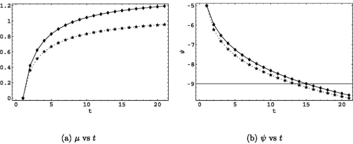
t 0, soA9d0. We henceforth drop the subscript onAd. See Fig. 1 for plots of the scale factor and dilaton in the distinct cases ofd3;9expanding dimensions; note that the time evolution of is not that sensitive to dimension.
As discussed in [14], the radiusRe asymptotes to the value
R1 e0
BpdA BpdA
1= d p
: (22)
Because the radius asymptotes to a finite value, the only hope that we have of ‘‘decompactification’’ of the
directions is for the string gas to leave the pressureless phase. As we have noted in our discussion of the thermo-dynamics, the gas of strings will leave the pressureless phase when the universe is no longer near the string radius, when e>R for some radius R which divides ‘‘large’’ from ‘‘small.’’ We take R 3 for numerical purposes. In particular, for the asymptotic radius R1>
R, we find that
e 0<_0 2d
E0
Re 0 d
p 1
Re 0 d
p 1
2
1
: (23)
As far as we know, this is the first discussion of such a
limit on the initial dilaton. Note that at large energies, the dilaton is considerably suppressed.
Finally, we should check that our initial conditions avoid a Jeans instability resulting in a black hole, as was discussed for string thermodynamics in [43]. To avoid the Jeans instability, we require
R2 1
"2#: (24)
For all radii initially atp0, (24) is
e 0 2 9
"2 0E0
: (25)
The constraint (25) is somewhat less restrictive than (23) if we keep _0<1 as required for the use of the
low-energy equations of motion.
B. Hagedorn strings at large radii
Now we would like to discuss the cosmological evolu-tion associated with a phase of strings at high energies and large radius, which we take to start at R >R. Although we will find later that the initial, pressureless phase cannot remain in equilibrium in order to lead to this phase, presumably strings could equilibrate after the universe reaches a large radius. Therefore, these cosmo-logical solutions may be useful in future studies. We know of no other reference that has considered the cosmologi-cal evolution of this phase of strings, as other works have concentrated on lower energy gases of strings, which are dominated by radiation (see [14,15,33]).
For this later era [39] give
0
E9e
0E$aRd (26)
for the multiple string density of states. We include the prefactor of 1=E9 because momentum and winding in
[image:4.612.130.488.541.687.2]each of the nine spatial directions are conserved, as discussed in [35,39]. Here $ is a constant (which we take to vanish), andais constant with radius but depends
on the number of large dimensions:
a 2d=2 2
d=2
d=2
Z1
0
dxxd1ln1 2
1p 2 1x 21=2:
(27)
The entropy is therefore
Sln09 lnE0E $aRd: (28)
The temperature and pressure are therefore
1
T
0E9
E ; (29)
P
E
0E9
$aded: (30)
Working with the usual assumption of adiabaticity, the equations of motion are now too difficult to solve analyti-cally. The main stumbling block is that, holding the entropy (28) fixed, the relation between the energy and radius is transcendent. However, it is straightforward to solve the equations of motion numerically; we found it useful to rewrite
1
dln
9 lnE
0ESln0
$a
; (31)
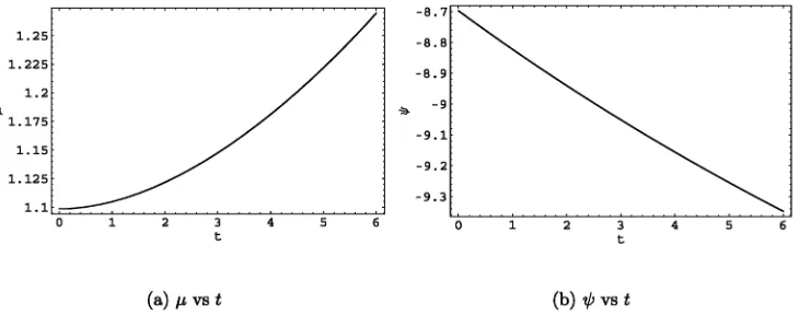
[image:5.612.50.297.69.248.2]and solve numerically forEas a function of time. We include plots of the scale factor and dilaton for this large-radius phase in d3 expanding dimensions in Fig. 2. For initial conditions, we take the values of E,
_
, , and _ given by evolving the pressureless phase to
eR3(although other initial conditions might be
more interesting, as indicated below). In the pressureless phase, we took the same initial conditions as listed in Fig. 1. Now the expanding dimensions can resume a rapid expansion, while the dilaton continues its monotonic decrease. When the energy density has decreased enough due to cosmological redshifting, this phase should match
onto a radiation dominated phase (assuming thermal equilibrium).
C. Estimating interaction rates from cosmology
Now we will consider the importance of (23) in deter-mining the interaction rate of strings. As a particular interaction of interest for the BV mechanism, we can focus on the annihilation of winding and antiwinding string pairs, although the key issue is whether the strings can remain in equilibrium. We first give a rough estimate of the interaction rate.
Up to gamma-function factors, the amplitude for any two-string to two-string process (with all dimensions near the string radius) ise , as we will discuss in more detail below. Therefore, we write the interaction rate roughly as
NX
s
X
~ p
e2 ; (32)
where N is the number of strings with which a given single string can interact, and the sums are over the outgoing spin and momentum states. At this level of discussion, the sum over spins just gives a constant factor of order 100. Also, for this simple estimate, we can approximate the sum over outgoing momentum states as a constant factor; for dimensions near the string radius, corresponding to the pressureless phase, this momentum sum factor is order unity.
Since the classical BV mechanism distinguishes the annihilation rates of winding strings in d3 and d >
[image:5.612.126.491.544.688.2]3 large dimensions, we comment here on the effect of varyingdon (32), the quantum mechanical annihilation rate. The dimensionality enters into through the time evolution of [and also somewhat in the constraint on its initial value (23)]; the higher d, the faster decreases. This effect tends to enact the BV mechanism, as strings interact less rapidly with more growing dimensions. The other factor through which daffects is the sum over outgoing momenta. Quite simply, for a given energy, the
phase space of outgoing momenta is larger in a greater number of large dimensions. This tends to counterbalance the variation of the dilaton, but it is a small effect when all dimensions are near the string radius.
The number of strings available for scattering is deter-mined by thermodynamics. For the pressureless phase, the number of strings of chargeqand energy between(
and(d(in a gas of strings of total energyEis [35]
N(; q; E
4
0
91
(
E
(E(
exp
E
4(E(q
TA1q: (33)
Here the matrixAis
A 0
42diag1|{z}=R;. . .
d
;1=R0;. . .
|{z}
9d
; R;. . .
|{z}
d
; R0;. . .
|{z}
9d
: (34)
This takes into account the contribution of winding and momentum, as well as oscillator modes, to the energy of the string. The total number of strings in the gas, given by summing over charge and integrating over (, is N
R
d(PqN(; q; E lnE. Actually, restricting to strings of a certain charge or range of energies gives a consid-erably smaller number, so we can takeN &lnE as an upper bound in (32).
If we substitute in the bound (23), our estimate of the interaction rate becomes
&100
_2 0d
E0
2
lnE0 (35)
during the entire pressureless phase. We have used the facts that the total energy in the string gas is constant during the pressureless phase and that the dilaton is monotonic decreasing. Even for E0 100, which only
leads to about four strings in equilibrium, we have<
_
0. For larger energies, the interaction rate will only
decrease.
Therefore, it seems inevitable that the string gas will fall out of equilibrium almost immediately as the uni-verse begins expanding in the pressureless phase. This means that, for anyd, winding strings will freeze out and come to dominate the energy density of the compact universe and cause its recollapse. Contrast this case to the original BV mechanism, which claims that winding strings can annihilate efficiently for d3.4The reader might wonder if the string gas could come into equilib-rium as _ decreases in time; however, if we assume pressureless evolution, _ /e while /e2 decreases
more rapidly.
As a result, any study of the standard BV scenario should focus on the nonequilibrium thermodynamics and cosmology of string gases, as partially discussed in [32,33] (these references included the nonequilibrium Boltzmann equation for strings but used the equilibrium cosmological evolution). There are a few possibilities to avoid this conclusion; however, they all modify the usual BV scenario. A simple idea would be to consider lower energy string gases (i.e.,0), as in [20], but winding
states would be populated only infrequently, so it might be difficult for winding strings to stabilize the radii of any of the dimensions. One obvious possibility is to take
_
01, which would require understanding the full
time-dependent world sheet conformal field theory (CFT). Unfortunately, this is beyond our capabilities, and in fact such a CFT may not have a straightforward geometric interpretation. Another possibility would be to consider the monotonically increasing solution for the dilaton, which could lead to a strong gravity regime and large time derivatives. Alternately, heterotic strings have qualitatively different thermodynamics due to additional low-energy states near the string radius, so they may evade (23). However, at high enough energies, even het-erotic compactifications should have a phase similar to the pressureless phase described above.
Another attractive option is the introduction of winding branes in the gas of strings, as has been widely considered [5–8]. Gases of D-branes might avoid our constraints because the branes couple to the dilaton and therefore modify Eq. (8). However, the other equations of motion remain the same [3], and, because brane gases are indeed T-duality invariant [6], the early phase of cosmology should still be pressureless. Therefore, _ /e as before. As long as decreases quickly enough, will still asymptote to a finite value, leading to a constraint on the initial value of the dilaton, as in (23). In a perturbative model, in fact, we expect D-brane states to be populated very little, so branes will not have much effect on the time evolution of . Therefore, it seems reasonable that (23) will hold approximately even if branes are included in the thermal gas of strings. See [11–13,16,17,19,21,22,25,26] for some work relevant to time evolution in brane gases. Similarly, allowing the shape moduli of the spatial torus and the various form fields of supergravity to be non-trivial may alter the qualitative behavior of the dilaton, such as by providing a potential (for a review of flux compactifications with stabilized dilaton, see [44]). Some work including other degrees of freedom in the context of string and brane-gas cosmology appears in [7,18,27,28]. We must caution that including a potential for the dilaton appears to prevent radius stabilization by winding strings, however [24].
As a final alternative, we propose a stochastic version of the BV scenario. In this case, we could imagine that the dilaton is large enough to maintain thermal equilibrium 4Of course, in more complicated compactifications, such as
of strings (so that the winding modes can annihilate), but the expanding dimensions asymptote to a small radius. Then, if some of these dimensions were to start expand-ing again due to some thermal or quantum fluctuation,
0>0, so the final radius (22) can grow. Eventually,
though a random walk, some dimensions could grow large while maintaining thermal equilibrium in the string gas. There are some difficulties with this proposal, however. One is understanding the quantum mechanics and thermodynamics of the supergravity background. Another is that the dilaton will still decrease monotoni-cally in time (except perhaps for thermal and quantum fluctuations), so the string gas might fall out of equilib-rium in any event.
All of the above proposals are candidates to allow the string gas to remain in thermal equilibrium and the wind-ing modes to annihilate. However, it is far from obvious that any of them discriminate among the number of expanding dimensions d. That is, in any of the above proposals, the values ofdwhich allow strings to remain in thermal equilibrium until all the winding strings an-nihilate (statistically speaking) seem likely to depend on initial conditions rather than d itself. Perhaps the most encouraging of our proposals in that regard is the inclu-sion of other form fields, which have varying rank, which could influence dimensionality to some extent.
III. INTERACTIONS IN TOTALLY COMPACT SPACES
In this section, we will calculate the annihilation rate for a winding and antiwinding string pair in order to confirm that the strings cannot stay in equilibrium in the pressureless phase. In so doing, we point out a problem with the naive use of string perturbation theory in the BV scenario and point out a resolution that could be useful in future tests of the BV mechanism.
As we have discussed, a key feature of the string-gas and brane-gas cosmologies is that all the spatial dimen-sions are compact; in fact, much of the interesting dy-namics that determines how many dimensions can expand to macroscopic size occurs when all the dimen-sions are within an order of magnitude of the string scale (loitering, for example, occurs at roughly2to3times the string length [25,26]). Because all the dimensions are compact and in fact at a small scale, momentum must be considered as being quantized. When the large dimen-sions become much larger than string scale, we are jus-tified in ignoring the momentum quantization because the energy spacing will be much smaller than other energy scales. However, since we are interested in string scale dimensions, the energy spacing of momentum modes is nearly as large as the string mass or even winding modes, we have to quantize momenta, even those in the large dimensions.
Quantization of all the momenta puts interesting con-straints on the interactions of strings, and, in particular, at generic compactification radii, interactions cannot con-serve energy. In other words, superstrings on a time-independentT9 (or presumably any other compact space)
cannot interact. To see this in more detail, consider some simple string amplitudes:
(i) Supergravity mode interaction in which two strings with momentum in thex1 direction scatter
into the x2 direction. In the simplest case, the
strings have no other momenta, so the initial strings have n1;n1 momentum numbers and
the final strings have n2;n2. Conservation of
energy would then require 2n1=R1 2n2=R2,
which is clearly impossible at generic radius since theni2Z.
(ii) Oscillator mode decay to momentum modes. If the final state strings have momenta in one direc-tion only, energy conservadirec-tion would requireN
2n=R, which is violated at nonintegral radius. (iii) Winding mode annihilation, which is our main
focus. In the simplest case, there are two strings with opposite winding number w;w in the x1
direction, which interact to produce, for example, momentum numbers n;n in the x2 direction.
Energy conservation would be 2wR1 2n=R2,
which is again clearly impossible for generic radii. In fact, even at radii (for example, R1) where the simplest case interactions listed above are allowed ener-getically, there are string states with multiple nonzero quantum numbers that cannot interact without violating energy conservation. Essentially, the problem is that at any given radius only a small subset of string interactions might be allowed by conservation of energy.
non-conservation of energy would average to zero over many interactions).
A. Time dependence and energy nonconservation
Because we have been careful to ensure that all time derivatives in the supergravity background are smaller than string scale, we can use a very simple approach to include the expansion of the universe in the string inter-actions. Namely, rather than incorporate time depen-dence directly into string perturbation theory, we develop an effective quantum mechanics based on string perturbation theory and then consider the time depen-dence of the effective quantum mechanics. We will focus on winding mode annihilation to momentum modes,
WW !NN, but our approach can easily be generalized to any interaction.
In its simplest form, we can take a two-state quantum mechanics, with the winding/antiwinding string pair (WW) as one state and the momentum string pair (NN) as the other. We derive the Hamiltonian as follows. The diagonal, mass part comes directly from the perturbative string spectrum on the fully compact space, and we do not need to discuss it further. Including an interaction piece, the Hamiltonian is
H 2jw~je VI
VI 2jn~je
; (36)
assuming that the momentum and winding vectorsn~and
~
ware completely in the expanding directions (the factors of 2 in the diagonal elements are because each state represents a pair of strings). To find VI, we compare to the corresponding amplitude 2.EfEiA for
WW !NN in string perturbation theory (which we dis-cuss in more detail in Sec. III B). Standard string pertur-bation theory assumes a time-independent background and allows an infinite time for the strings to interact. In quantum mechanical perturbation theory in this case, we find the same amplitude
hn;~ n~jw;~ w~i iZ dt0eiEfEit0V
I
iVI2.EiEf; (37)
for a time-independentVI. Taking into account the rela-tivistic normalization of states in string perturbation theory,
VI A
Q4
i12Ei
q ; (38)
where the Ei are the energies of the incoming and out-going strings. Extracting the dependence on supergravity fields,VI Ce , where
C e
A
2E12E22E32E4
p (39)
is a constant factor. One advantage of this effective quan-tum mechanics approach is that the string amplitude automatically includes single string intermediate states, as we will discuss in more detail below. To include the evolution of the universe at any given time t0, we can expandHto first order in time derivatives,HH0Ht. Then we can treat the first order term as a perturbation around the zeroth order term.
We should therefore first find the eigenstates of the time-independent Hamiltonian, including the interac-tionsVI. In this way, we avoid confusing state oscillation of the purely time-independent quantum mechanics in the annihilation rate, which should be due purely to time dependence in the Hamiltonian. Using standard formulas from quantum mechanics (see, for example, [45]), the eigenstates are given by
jw;~ w~i jw;~ w~i0 VI
E0
wE0n
jn;~ n~i0;
jn;~ n~i jn;~ n~i0 VI
E0
nE0w
jw;~ w~i0;
(40)
where the energy eigenvalues are just the unperturbed onesE0
w; E0n. We have treatedVI as a perturbation because we are working in a regime in which string perturbation theory is valid ( <0).
The lowest order transition amplitude for winding annihilation is (again, see [45], for example)
c1 i
Ce _ 1
!2Ce we_
1
!2Ce ne
_
tei!t
i!
ei!t1
i!2
; (41)
with
!EfEi2n
R 2wR: (42)
Here,n jn~jandw jw~j.
Next we note thatt;_ t <_ 1in order to ensure that we can treat the time dependence as a perturbation. In fact, this is consistent with assumingt 1for the interaction time of strings, as the supergravity approximation re-quires that all time derivatives be less than unity. Then we can take!tto be small, so the probability is therefore
P jCe j2_ 2
4
we_ _
!
_
ne _
!
w2_2e2
!2
2wn_
2
!2
_
2n2e2 !2
t4: (43)
The total annihilation rate for a winding string (WW !NN), as discussed in Sec. 4 following Eq. (32), is
NX
s
X
~ n
Pw; ~~ n; (44)
polar-izations for simplicity, the sum over outgoing spins re-duces to an overall constant. In fact, conservation of angular momentum correlates the two outgoing spins, so the overall factor will be the number of massless superstring spins,256, times a symmetry factor of1=2. The sum over outgoing momenta should be within the (larger) expanding dimensions, as that is the type of final state that interests us. Before we present the results of a detailed computation, we will discuss the string pertur-bation theory amplitude A that we used to define the effective quantum mechanics.
One note: The reader may wonder why we did not take advantage of the optical theorem to calculate the total interaction rate (up to the factor ofN), as in [32,46,47]. The simple reason is that we have no simple way to incorporate the time dependence of the background into the appropriate calculation in string perturbation theory, unlike the direct calculation that we present.
B. Bosonic string winding annihilation amplitude
As we discussed above, we need the string perturbation theory interaction amplitude. We carry out a somewhat rough analysis of the interaction, ignoring the contribu-tion to the amplitude from string polarizacontribu-tions. This approximation allows us to replace the sum over outgoing spins by an overall factor (and the average over incoming spins by unity) in the interaction rate (44). Therefore, we use the bosonic string amplitude for nonpolarized strings (the tachyon mode if the winding and compact momenta vanish) but with the appropriate mass-shell for whatever polarized superstring modes we are considering. An analogous superstring calculation for tachyonic winding strings was discussed in [47] using the optical theorem; we calculate the amplitude directly at tree level for use in the effective quantum mechanics as discussed above. Our presentation is a generalization of the answer to a text-book problem from [48].
In calculating the annihilation amplitude, we find it convenient to work with a unit metric and coordinate radii equal to the proper radii of the spatial dimensions, but the amplitude is diffeomorphism invariant and can therefore be used directly with the conventions in the text. The vertex operators of the four interacting strings are all
gc
V
p :expik
LXLikRXR:; (45)
where the closed string coupling
gc 1
2
p 25=2 02e4; (46)
4 is the 10D dilaton, and V is the total volume of the spatial dimensions (the product of 2R over all dimensions). The amplitude is just the expectation value of four vertex operators, and it has a prefactor (besides the vertex operator normalization) of
i8=g2
c 02.Pk0V.n.w. Here .Pk0 conserves energy and.n;wconserve compact momentum and wind-ing (i.e., these are products of Kronecker delta symbols). There is also an overall sign (the cocycle) which we will ignore as we have only a single amplitude. Thus, the amplitude becomes
A i223e 2.10dk.
n.wFkL; kR; (47) with as before. HereFis some function of the momenta that we need to determine, and we are again setting
0
1.
As it turns out, we are interested in annihilation of winding, so the two outgoing strings will have zero wind-ing, and the two incoming strings will have opposite winding w~ w~1 w~2. In addition, we will take the simplest case in which the winding strings have no mo-mentum. The compact momenta are
~
kL3k~R3 k~L4 k~R4
n
R
!
;
~
kL1 k~R1 k~L2k~R2 wR;
! (48)
where n=R! is the vector with componentsni=Ri(Ri is the physical radius in theith direction) and similarly for
wR!. Additionally,k0I represents theincomingenergy of theIth string, which is negative for the outgoing momen-tum strings, while EI is the physical energy of the Ith string, which is always positive.
In this case, the momentum dependence becomes
FZ d2zjzjE1E4j1zjE2E4
z
z
n~w=~ 21z
1z
n~w=~ 2
(49)
integrated over the sphere. Note that E3;4 appear
asym-metrically due to the way in which we have located the vertex operators on the sphere; however, the end result will be symmetric, as it must due toSL2;Cinvariance on the world sheet. To do this integral, we can integrate by parts n~w~ on each of z. Then we find some prefactors along with the usual integration needed for the Virasoro-Shapiro amplitude. As it turns out, the functions from the integral can absorb the prefactors, giving us
FF1F2F3;
F11
1
2E1E4n~w~
1
2E1E4n~w~
1
1
2nwn~w~
1
2nwn~w~
;
F2
11
2E2E4n~w~
1
2E2E4n~w~
1
1
2nwn~w~
1
2nwn~w~
;
F3
11
2E1E2E4 21
2E1E2E4
1nw
2nw : (50)
the form (in the general case)
E24Nn
R
! 2
wR!2: (51)
N is an integer that describes the oscillator excitation of the string. For bosonic string tachyon vertex operators, such as we are using, we should takeN 1; however, we want to simulate superstrings at the massless level, so we takeN0. We have therefore takenE1;2 wRand
E3;4 n=R.
There is one additional subtlety to discuss. By unitar-ity, the string amplitude contains poles corresponding to single string intermediate states. (This fact is actually very useful for our quantum mechanics because it means we do not need to use second order perturbation theory to include all interactions at the same order ine . All the tree-level annihilation processes are included in this single sphere amplitude.) These poles appear through the gamma function in the numerator of F3, which has
a pole whenevernwis an integer. Indeed, if we rewritenw
in terms of the center-of-mass energy (Mandelstam vari-able) nws=4 E1E22 E
3E42, then the
poles are at s 4;0;4;8;. . ., just the bosonic closed string oscillator spectrum.
However, since we are interested in computing the actual interaction rates, we must include the widths of the poles. Although we do not know the appropriate formulation of resonances in the full time-dependent formalism, we can, at our level of approximation, use the traditional Breit-Wigner resonance, replacing s!
simw at the pole given bysm2, where w is the width of the resonance (see a quantum field theory text, such as [49]). To encompass all the poles at once, we use
s!sipsw, which is correct at each pole. To calculate the width, we ignore string polarizations again, so the width becomes
w128
X
~ n
1 2ps
1
s
8
22e .
s
p
2n=R: (52)
The delta function conserves energy, andpsis the energy of the intermediate oscillator resonance. Because of mo-mentum conservation, the sum over outgoing momenta is a single sum in the d expanding directions, which we approximate by an integral:
X
~ n
.ps2n=R RdZ ddp.~ ps2jp~j
R d
2
s
p
2
d1 2d1=2
d1=2: (53)
Therefore, the width is
w 64Rde s
4
d4=2 2d5=2
d1=2; (54)
leaving us
F3
1nwipnww=2
2nw ; (55)
withsreplaced by4nwinw.
C. Results of calculation
We now briefly present the results of calculating the total annihilation rate (44) in the pressureless phase of the cosmology. For the purposes of the calculation, we first takeN N(wR; qw; E~ (, where we take
(1 in string units. Thus, we are calculating the annihilation rate purely for strings withw~ units of wind-ing and no extra oscillators. Then, as an upper bound on the annihilation rate, we take N lnE, which is the total number of strings in the thermodynamical gas. We see that, in either case, the interaction rate is small compared to the Hubble constant_, so the gas must fall out of equilibrium. We do the momentum sumPn~by brute force, requiring at all times that the frequency !
2n=R2wR <1 (since larger values are suppressed). For our example calculation, we take w~ 1;0;0 . . . 0, andR3in the first era, so we take each component ofn~
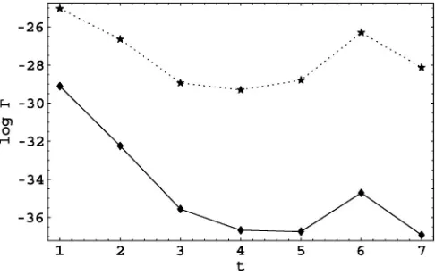
between 10 and 10 for the sum over momenta. The logarithm of the interaction rate is plotted in Fig. 3. The initial conditions are the same as those used in plotting Fig. 1. Note that the gamma functions give an additional suppression of the interaction rate.
The interaction rate is very small compared to the Hubble parameter (which is order unity as an initial condition). We have carried out this calculation also for
[image:10.612.318.561.512.666.2]d2;4expanding dimensions and found no qualitative difference. There is one interesting feature of these inter-action rates: a slight increase at later times. This tempo-rary increase is due to an increase in phase space available to the outgoing modes as some of the dimensions expand.
FIG. 3. The interaction rate for strings in the pressureless phase for d3expanding dimensions. The initial conditions are those given in Fig. 1. The lower, solid curve has N
IV. SUMMARY
In summary, we have made two arguments regarding the usual Brandenberger-Vafa proposal for the cosmology of string gases on totally compact spaces.
In the first part of the paper, we analyzed two possible states of a string gas at high energies, reviewing their thermodynamics and solving for the cosmological evolu-tion of the universe in those phases. The later phase had not been previously studied in the literature. From the time evolution of the dilaton and scale factor, we were able to give a heuristic argument that there are not initial conditions in the small-radius, pressureless phase that both grow into the large-radius phase and maintain ther-mal equilibrium of the string-gas. We also argued that more general brane gases would likely have a similar constraint and gave several possible scenarios that could avoid this conclusion, all of which modify the usual Brandenberger-Vafa scenario. One key point is that our conclusion that strings fall out of thermal equilibrium is largely independent of the number of expanding dimen-sions. Therefore, it would seem like any possible modifi-cation to the Brandenberger-Vafa scenario would not select a favored number of large dimensions, as was originally proposed in [1].
In the second part of this paper, we calculated the approximate annihilation rate for winding strings in dif-ferent numbers of expanding dimensions. This calculation confirmed that the strings cannot remain in thermal equi-librium in the small-radius phase of the string gas. In that section of the paper, we also argued that quantization of string momenta is important during the small-radius phase. Specifically, due to quantization of string winding and momenta, string interactions will generically violate conservation of energy (and would thus seemingly be forbidden). We demonstrated that the time dependence of the supergravity background allows string interactions even at small radii, using time-dependent perturbation theory in an effective quantum mechanics. We believe this approach will be useful in future studies of small-radius Brandenberger-Vafa cosmology.
In conclusion, then, we have argued that it seems un-likely that string-gas cosmology in totally compact spaces provides an explanation for the number of macro-scopic dimensions, especially when our work is taken in concert with [31– 33]. Nonetheless, the Brandenberger-Vafa proposal is a very natural initial condition for cos-mology from the point of view of string theory, so it is worthy of continued study. We have in fact given some directions which we believe would be interesting for future work.
ACKNOWLEDGMENTS
We would like to acknowledge comments from R. Brandenberger and M. Sheikh-Jabbari and useful
con-versations with J. Polchinski and especially P. Kraus. The work of ARF has been supported by a John A. McCone Fellowship in Theoretical Physics at the California Institute of Technology.
APPENDIX: QUANTUM RADII
In this appendix, we would like to sketch another approach to resolving issues of energy conservation in completely compact spaces based on elementary consid-erations of quantum gravity. In quantum gravity, we should really consider the metric to be some quantum variable, so that the radii of the compact dimensions should not be fixed to the classical cosmological trajecto-ries. Rather, there should be a wave function !; giving the probability density for different values of
; , which should be peaked at the classical trajectory. In fact, in the perturbative string regime, we expect that these are sharp peaks because the Planck mass is very large (even compared to the string scale). (We expect that
!is most simply written in terms of; because those variables have canonical kinetic terms.)
Then the total state of the system (at fixed time) should be described as jfmatterg; ; i, where the matter part describes whatever string might be currently in the uni-verse. For simplicity, all but two of the strings will be taken to be spectators (as is usual in perturbation theory), and they will give only a factor of unity. Therefore, the total amplitude A hfmatterg; ; jfmatterg; ; i should be
A Z ddj!; j2A^ .XE; : (A1)
Here,A^ is a reduced string amplitude; just the amplitude from string perturbation theory with the energy conserv-ing delta function extracted. We will take the wave func-tion to factorize on ; . To simplify notation, we will henceforth letEbe the sum over energies (with outgoing energies taken to be negative). As an aside, we are ignor-ing any complications to the measure caused by our constraining sets of dimensions to have the same radii.
Then suppose we have the simple case described above for winding mode annihilation. If both the winding and momentum directions have the same radius (i.e., both are among the large dimensions represented by ), we can evaluate the integral easily to get
A 1
4pnw
!
1
2ln
n w
2 ^
A: (A2)
Here we have integrated over the dependence of the wave function. Other examples proceed in the same way, with a slight complication if the energy depends on both
A Z dj!; j2
@E
@;
1
^
A; ; (A3)
where is the value of that satisfies conservation of energy as a function of. If the wave function is sharply peaked in, then
A ’ j!j2
@E
@
1
^
A; (A4)
where ! now depends only on and everything else (including) are evaluated at the peak (classical) value of.
The interaction probability should be given by the normalized square of the amplitude, as usual. To get the rate, however, we must divide the probability by the amount of time over which the interaction has been allowed to take place. In perturbative string theory, as in perturbative field theory, we have essentially assumed that strings have been allowed to interact over some long period of time. Usually, the square of the amplitude has two energy conserving delta functions, and one of those delta functions, evaluated at zero, becomes the interaction time. In our analysis, the radial wave function replaces the energy conserving delta function and should also repre-sent the interaction time.
We can understand this fact by considering the classical limit of our amplitude. If we turn off quantum gravity (perhaps by sending the dimensionally reduced dilaton ! 1), then we should have j!; j2 . ^
.^, where ;^ ^ are the classical values. Then we obviously get the usual amplitude. However, we can
also integrate over ; , so the amplitude is as in (A4). Then we note that
j!j2@E
@
1
. ^
@E
@
1
.E^: (A5)
Therefore, when we square the amplitude, we have two factors of j!j2=@E=@, one of which should be
eval-uated at the classical values;^ ^ and divided out to give the rate.
Once we average over incoming polarizations and sum over outgoing states, we end up with a rate
NX
s
X
~ n
j!; ^j2@E
@; ^
1
jA^ w~i; ~ni; ~no;; ^j
2
2E1 2E4 : (A6)
Here the notation is as in Eq. (44), and we have speci-alized to the two-string annihilation or scattering rate.
What is missing from this prescription is a wave func-tion for the radii, as well as its dynamics. One particu-larly important question is how each string interaction affects the wave function; that is, does the string interac-tion ‘‘collapse’’ the wave funcinterac-tion or is there some more complicated entanglement or decoherence process? Another point concerns the quantum mechanical evolu-tion of the wave funcevolu-tion. For example, if we choose to model the wave function as a Gaussian, how does the width of the Gaussian evolve with time?
[1] R. H. Brandenberger and C. Vafa, Nucl. Phys.B316, 391 (1989).
[2] A. A. Tseytlin and C. Vafa, Nucl. Phys.B372, 443 (1992). [3] A. A. Tseytlin, Classical Quantum Gravity 9, 979
(1992).
[4] M. Maggiore and A. Riotto, Nucl. Phys. B548, 427 (1999).
[5] S. Alexander, R. H. Brandenberger, and D. Easson, Phys. Rev. D62, 103509 (2000).
[6] T. Boehm and R. Brandenberger, J. Cosmol. Astropart. Phys. 06 (2003) 008.
[7] S. H. S. Alexander, J. High Energy Phys. 10 (2003) 013. [8] D. A. Easson, Int. J. Mod. Phys. A18, 4295 (2003). [9] R. Easther, B. R. Greene, and M. G. Jackson, Phys. Rev. D
66, 023502 (2002).
[10] R. Easther, B. R. Greene, M. G. Jackson, and D. Kabat, Phys. Rev. D67, 123501 (2003a).
[11] S. Watson and R. H. Brandenberger, Phys. Rev. D 67, 043510 (2003).
[12] S. Watson and R. Brandenberger, J. Cosmol. Astropart. Phys. 11 (2003) 008.
[13] R. Brandenberger, D. A. Easson, and A. Mazumdar, Phys. Rev. D69, 083502 (2004).
[14] B. A. Bassett, M. Borunda, M. Serone, and S. Tsujikawa, Phys. Rev. D67, 123506 (2003).
[15] M. Borunda, hep-th/0310032.
[16] A. Kaya, Classical Quantum Gravity20, 4533 (2003). [17] A. Campos, Phys. Rev. D68, 104017 (2003).
[18] S. Watson and R. Brandenberger, J. High Energy Phys. 03 (2004) 045.
[19] A. Kaya, J. Cosmol. Astropart. Phys. 08 (2004) 014. [20] S. P. Patil and R. Brandenberger, hep-th/0401037. [21] T. Battefeld and S. Watson, J. Cosmol. Astropart. Phys. 06
(2004) 001.
[22] J. Y. Kim, hep-th/0403096.
[23] S. Arapoglu and A. Kaya, hep-th/0409094. [24] A. J. Berndsen and J. M. Cline, hep-th/0408185.
[25] R. Brandenberger, D. A. Easson, and D. Kimberly, Nucl. Phys. B623, 421 (2002).
[26] D. A. Easson, hep-th/0111055.
[29] A. Campos, hep-th/0409101.
[30] M. Sakellariadou, Nucl. Phys. B468, 319 (1996). [31] G. B. Cleaver and P. J. Rosenthal, Nucl. Phys.B457, 621
(1995).
[32] R. Easther, B. R. Greene, M. G. Jackson, and D. Kabat, J. Cosmol. Astropart. Phys. 01 (2004) 006.
[33] R. Easther, B. R. Greene, M. G. Jackson, and D. Kabat, hep-th/0409121.
[34] N. Deo, S. Jain, and C.-I. Tan, Phys. Lett. B 220, 125 (1989).
[35] N. Deo, S. Jain, and C.-I. Tan, Phys. Rev. D 40, 2626 (1989).
[36] M. J. Bowick and S. B. Giddings, Nucl. Phys. B325, 631 (1989).
[37] N. Turok, Physica A (Amsterdam)158, 516 (1989). [38] N. Deo, S. Jain, and C.-I. Tan, in Proceedings of the
International Colloquium on Modern Quantum Field Theory, Bombay, India, 1990, edited by S. Das, A. Dhar, S. Mukhi, A. Raina, and A. Sen (World Scientific, Singapore, 1991).
[39] N. Deo, S. Jain, O. Narayan, and C.-I. Tan, Phys. Rev. D 45, 3641 (1992).
[40] J. L. F. Barbon and E. Rabinovici, hep-th/0407236. [41] K. H. O’Brien and C. I. Tan, Phys. Rev. D 36, 1184
(1987).
[42] E. Alvarez and M. A. R. Osorio, Phys. Rev. D36, 1175 (1987).
[43] J. J. Atick and E. Witten, Nucl. Phys.B310, 291 (1988). [44] A. R. Frey, hep-th/0308156.
[45] J. Sakurai, Modern Quantum Mechanics (Addison-Wesley, Reading, MA, 1994).
[46] J. Polchinski, Phys. Lett. B209, 252 (1988).
[47] M. G. Jackson, N. T. Jones, and J. Polchinski, hep-th/ 0405229.
[48] J. Polchinski, String Theory (Cambridge University Press, Cambridge, United Kingdom, 1998).