High frequency variability and microstructure bias

High Frequency Variability and Microstructure Bias

Adam Sykulski∗

Dept. of Mathematics, Imperial College London

SW7 2AZ, London [email protected]

Sofia Olhede†

Dept. of Statistical Science University College London

WC1 E6BT, London [email protected]

Grigorios Pavliotis‡

Dept. of Mathematics, Imperial College London

SW7 2AZ, London [email protected]

Abstract

This paper treats the multiscale estimation of the integrated volatility of an Itˆo process immersed in high-frequency correlated noise. The multiscale structure of the problem is modelled explicitly, and the multiscale ratio is used to quantify energy contributions from the noise, estimated using the Whittle likelihood. This problem becomes more complex as we allow the noise structure greater flexibility, and multiscale properties of the estimation are discussed via a simulation study.

1

Introduction

The estimation of properties of continuous time stochastic processes, whose observation is immersed in high frequency nuisance structure is required in many different fields of application, for example molecular biology and finance. Various methods have been proposed to alleviate bias introduced into the estimation from high frequency nuisance structure, see for example [1–4]. Commonly the model of the observed process is as the process of interestXtisuperimposed with noiseti, or

Yti =Xti+ti, (1)

whereYti is the observed process, Xti the unobserved component of interests, andti is the

mi-crostructure noise effect. We modelXt, the process of interest with a suitable stochastic differential

equation. For example, the Heston model is specified [5] by

dXt= (μ−νt/2)dt+σtdBt, dνt=κ(α−νt)dt+γνt1/2dWt, (2)

whereνt=σt2, andBtandWtare correlated 1-D Brownian motions.

Our main objective is to estimate the integrated volatility,_hX, X_iT of the Itˆo process{Xt}, from

the set of observations_{Yti}. Different methods have been proposed for determining the properties

ofXti. An outstanding problem is proposing more robust inference methods. [3] has relaxed the

assumptions of [1], to include inference of processes with jumps. Another possible direction of de-velopment is to include more complicated noise scenarios, namely allowing for correlation between observations. The main issue with such relaxations, is that as the permitted structure ofXtand

tbecome less stylized, it naturally becomes harder to separate energy due to the high frequency

nuisance component from the process of interest.

Sykulski et al. [4] have proposed inference for multiscale processes based on using the discrete Fourier transform. Fourier domain estimators have also been used for estimating noisy Itˆo pro-cesses, see [6], but the main innovation of Sykulski et al. was to present a theoretical framework for Harmonizable processes [7, 8] of interest, and an automatic procedure for estimating the nuisance structure was proposed. The Whittle likelihood was used to estimate the energy level of the process of interest, as well as the noise contamination. The method was shown to perform well under various signal to noise scenarios, as well as path lengths, see [4].

The results of [4] or [1] are only appropriate when the noise is white. We shall in contrast in this paper discuss possible extensions of the multiscale estimators to the case of more complicated market microstructure, and illustrate the performance of the estimator in various noise scenarios.

2

Multiscale Estimation

In the absence of noise a suitable estimator of the integrated volatility,_hX, X_iT =R₀Tσt2dt, can be

specified from the quadratic variation of the process_{Yt}. In the presence of market microstructure

noise this is no longer true and it is necessary to employ a different estimation procedure. For ease of exposition we denote the difference processZti−Zti−1 byU

(Z)

ti whereZ =X,Y or. The

Lo`eve spectrum [7,8] ofU_t(Z)_i will be denotedS(Z)_(f

k, fk), and we note that the observed quadratic

variation can be rewritten as:

\

hX, X_i(b)_T =

N_X−1

i=0

U_t(Y_i )2=

N/2−1

X

k=−N/2

J(Y)(fk)

2 (3a)

b

S(Y)(fk, fk) =

J(Y)(fk)

2, J(Y)(fk) = √1

N

N_X−1

j=1

U_t(Y_j )e−2πitjfk_{. (3b)}

withfk = _Tk.Sb(Y)(fk, fk)is the periodogram estimator, see [9], and normally has a single

argu-ment because the covariance of the Fourier Transform at two fixed frequencies is asymptotically equivalent to zero for a stationary process. We note directly from [4] that the bias of the estimator

\

hX, X_i(b)_T is conveniently expressed in the Fourier domain by the observation that

E

\

hX, X_i(b)_T

=

N/2−1

X

k=−N/2

S(X)(fk, fk)+σ2 N/2−1

X

k=−N/2

|2 sin(πfkΔt)|2+O(Nα)+O N1−α

. (4)

The error terms follow from assumptions regarding the spectral properties of the processXt, and are

detailed in [4]. These assumptions determine the value ofα. It is clear from eqn (4) that the influence of the noise increases for larger frequencies, and that the relative magnitude ofS(X)_(f

k, fk)to

σ2

|2 sin(πfkΔt)|2at frequencyfkwill determine the need for bias correction atfk.

Sykulski et al proposed to measure the average energy ofU_t(X)across frequencies, and determine the energy ofU_t(), using the form of the white noise spectrum. DespiteU_t(X)assumed harmonizable and not necessarily stationary, with appropriate assumptions regarding the spectral correlation of the process, it is appropriate to use the Whittle likelihood, see [10], to determine the relative energy of the two processes across scales. Instead of using eqn (3b) to estimate the spectral contributions of the process of interest, a shrinkage estimator ofS(X)_(f

k, fk)was therefore proposed in [4]:

b

S(X)(fk, fk;Lk) =LkSb(Y)(fk, fk). (5)

0 _≤Lk ≤1is referred to as the ‘multiscale ratio’ and its optimal form for perfect bias correction

whentiis white noise is given by:

Lk=

S(X)_(f k, fk)

S(X)_(f

k, fk) +σ2|2 sin(πfkΔt)|2

. (6)

Of course this assumes perfect knowledge ofS(X)_(f

k, fk)and is not a realizable estimator. Instead

typical contributions ofS(X)_(f

k, fk)across frequencies were considered, and the multiscale ratio

replaced by a sort of average ratio corresponding to

Lk =

σ2 X

σ2

X+σ2|2 sin(πfkΔt)|2

. (7)

The justification for this choice is discussed in Sykulski et al. We estimate the parameters ofLk

σ= σ2 σ2_X

`(σ) =₋

N/_X2−1

k=1

log σX2 +σ2|2 sin(πfkΔt)|2

− N/_X2−1

k=1

b

S(Y)(fk, fk)

σ2

X+σ2|2 sin(πfkΔt)|2

.

If

n

U_t(X)o is a stationary process, then the full Whittle likelihood (with σ2

X replaced by

S(X)_(f

k, fk)) will approximate the time-domain likelihood of the sample, under suitable regularity

conditions, see [11].

The bias corrected estimator of the integrated volatility for an estimatedLˆKsequence becomes

\

hX, X_i(m_T 1)=

N/2−1

X

k=−N/2

b

S(X)(fk, fk;Lbk). (8)

In Sykulski et al. it was shown that the estimates ofσ2

Xandσ2produced suitableLbk such that bias

corrected estimators ofS(X)_(f

k, fk)with suitable properties were defined. Unfortunately it is not

always reasonable to model the high frequency structure as white, and so more subtle modelling needs to be used when the noise is more complicated.

3

Correlated Noise

A key issue is treating correlation in the error terms. A reasonable relaxation of modelling ti

as white would correspond toti stationary. Stationary processes can be conveniently represented

in terms of aggregations of uncorrelated white processes, using the Wold decomposition theorem [12][p. 187]. We may therefore write the zero-mean observationtias

ti =

∞

X

j=0

θtjηti−tj, (9)

whereθt0 ≡1,

P

jθ2tj <∞,and{ηtn}satisfiesE [ηtn] = 0andE [ηtnηtm] =σ

2

ηδn,m. Common

practise would involve approximating the distribution by a finite number of elements in the sum, and thus truncate eqn (9) toq _∈Z. We therefore model the noise as a Moving Average (MA) process specified by

ti=ηti+

q

X

k=1

θtkηti−k, (10)

and the spectral density function [9] oftitakes the form:

S∗(f;θ, σ_η2) =σ2_η 1 +

q

X

k=1

θke2iπf k

2

. (11)

In this case our spectral model fortichanges to a Lo`eve spectrum of

S()(f, f) =S∗(f;θ, σ2_η)|2 sin (πfΔt)|2_{. (12)}

Two possible methods now exist for treating the nuisance function ofS∗_{(f;θ, σ}2

η): we can use the

method of Sykulski et al. directly without adjustment, assuming the variability ofS∗_{(f;θ, σ}2 η)to

be moderate or we could adjust the methodology to encompass a parametric model for the noise, replacingσ2

|2 sin (πfΔt)|2byS∗(f;θ, σ2η)|2 sin (πfΔt)|2when treating the frequency structure

of the micro structure noise.

For a fixed and specified value ofq, we may therefore estimate the parameters of the MA, using the Whittle likelihood, but where nowσ2

thus get a multiscale likelihood1given withσ= σ2_η σ2_Xby

`(σ,θ) =₋

N/2−1_X

k=1

logσ_X2 +S∗(fk;θ, σ2η)|2 sin(πfkΔt)|2

−

N/2−1

X

k=1

b S(Y)_(f

k, fk)

σ2

X+S∗(fk;θ, ση2)|2 sin(πfkΔt)|2

. (13)

and the augmented multiscale ratio is defined by

L(a)_k = σ

2 X

σ2

X+S∗(fk;θ, ση2)|2 sin(πfkΔt)|2

. (14)

Ifqis not assumed known, then model choice methods can also be applied to determine the value ofq, such as applying the modified Akaike AIC [12][p. 287], and adding2n(q+ 2)/[n₋q₋3]to minus two times the log multiscale likelihood, and minimizing this objective function. Some care must be applied as the Akaike AIC is known to overestimate the number of parameters, and BIC or some other model choice method may be applied. For a chosen value ofqonce we augment the estimation ofσ2

Xandσ2with that of{θtk}, then we can estimate the noise spectrum and hence the

multiscale ratio. This will yield an augmented estimator of the integrated volatility, replacing the parameters by their estimators in eqn (14), that we denote byLb(a)_k . Our new estimator then takes the form

\

hX, X_i(a)_T =

N/2−1

X

k=−N/2

b

S(X)(fk, fk;Lb(a)_k ). (15)

This form both takes the high frequency structure into account, and permits the high frequency structure to be more dynamic than is the case of simple white noise nuisance structure.

4

Examples

We investigate the simple case of

ti=ηti+θ1ηti−1, (16)

where then S∗_{(f) = 1 +θ}2

1 + 2θ1cos(2πf). Clearly it is of interest to investigate the effect

of the variability ofS∗(f)on the multiscale estimation procedure. We note that settingθ1 = 0

recovers the white noise structure investigated in [4] and [1]. It is therefore of interest to compare our estimators over a range of values forθ1to study the effect of additional variability in the spectrum

of the nuisance structure in the estimation of the integrated volatility. This is not a full study of the complete effects of complicated high-frequency structure superimposed on the process of interest: this study is intended to demonstrate the adverse effects of a more dynamic nuisance structure, and the potential of correcting for such effects using the multiscale structure of the process of interest.

We demonstrate the performance of our multiscale estimators of integrated volatility using the He-ston model defined in eqn (2), with the same parameter values as used in [4] and [1], except this

time we generate the microstructure noise process by eqn (16). Our new estimator _h\X, X_i(a)_T , requires estimation of the parameters (σ2

X, σ2, θ1) and this is done separately for each path

us-ing the MATLAB functionfmincon on eqn (13). Figures 1(a) and 1(b) show the approximated

σ2_XandS∗(fk;θ1, ση2)|2 sin(πfkΔt)|2(in white) plotted over the periodogramsSb(X)(fk, fk)and

b S()_(f

k, fk)for one simulated path, whereθ1 = 0.5. The parameters(σX2, σ2, θ1)seem to have

been approximated well, as the approximated spectral densities follow the shape of their respective periodograms. Figure 1(c) shows the corresponding multiscale ratioLb(a)_k (in white) plotted over an unrealizable estimate ofLk:

e

Lk=

b S(X)_(f

k, fk)

b S(X)_(f

k, fk) +Sb()(fk, fk)

. (17)

1

Table 1: Root Mean Square Error (RMSE) for the different estimators of the integrated volatility, over different values ofθ1. The RMSEs are averaged over 7,500 paths.

RMSE_{{∙} h}\X, X_i(b)_{T h}\X, X_i(s_T1) _h\X, X_i(m_T 1) _h\X, X_i(a)_{T h}\X, X_i(u)_T

θ1=−1 3.51×10−2 4.82×10−4 7.35×10−5 1.52×10−5 1.46×10−5

θ1=−0.75 2.71×10−2 3.62×10−4 7.14×10−5 1.56×10−5 1.44×10−5

θ1=−0.5 2.05×10−2 2.42×10−4 6.40×10−5 1.57×10−5 1.44×10−5

θ1=−0.25 1.54×10−2 1.21×10−4 4.58×10−5 1.60×10−5 1.44×10−5

θ1= 0 1.17×10−2 1.67×10−5 1.61×10−5 1.62×10−5 1.43×10−5

θ1= 0.25 9.51×10−3 1.22×10−4 1.18×10−4 1.67×10−5 1.45×10−5

θ1= 0.5 8.78×10−3 2.41×10−4 4.67×10−4 1.70×10−5 1.43×10−5

θ1= 0.75 9.51×10−3 3.62×10−4 2.13×10−3 1.74×10−5 1.44×10−5

θ1= 1 1.17×10−2 4.82×10−4 9.82×10−3 1.67×10−5 1.45×10−5

Our multiscale ratio provides a good estimate toLk and will remove the noise microstructure from

the correct frequencies by shrinkage. Figure 1(d) shows Lb(a)_k Sb(Y)_(f

k, fk); the energy has been

shrunk at frequencies affected by the microstructure noise and the spectrum is a good approximation toSb(X)_(f

k, fk), which in turn should lead to a good approximation of the integrated volatility,

compare with Figure 1(a). Figures 2(a) and 2(b) show two more estimated multiscale ratiosLb(a)_k (in white), but this time withθ1 =−0.5andθ1 = 1respectively. The multiscale estimator appears to

correctly detect the correlation of noise in the process, as well as the magnitude of the signal to noise ratio. Note that forθ1=−0.5we shrink the estimated Lo`eve spectrum at an increasing rate for high

frequencies, whilst forθ1= 1we shrink in a highly non-monotone fashion across frequencies.

We investigate the performance of our new estimator against the estimators developed in [4] and [1] using Monte Carlo simulations. A range of values forθ1 are used to investigate the effect of

correlated noise. For each value ofθ1 we generated 7,500 simulated paths. Table I displays the

results of our simulation, where the errors are calculated using a Riemann sum approximation on

theXt process (see [4] for details). Along with the performance of our new estimatorh\X, Xi (a) T

(eqn (15)), we include the performance of the estimator from [4],_h\X, X_i(m_T 1) (eqn (8)) and the

best un-biased estimator developed in [1], _h\X, X_i(s_T1). Naturally we do not aim to compare our estimator for correlated noise structure with that of [1, 4], as these were not developed for correlated noise, but more include these to show the necessity of treating correlation in the microstructure. Furthermore, had our Whittle estimators been sufficiently poor, then the variability of the estimated multiscale ratio would have made our proposed procedure unsuitable. We also include for reference,

the biased estimator in eqn (3a), _h\X, X_i(b)_T (the quadratic variation on Yt) and the unobservable

unbiased estimator

\

hX, X_i(u)_T =

N_X−1

i=0

U_t(X)_i 2 (18)

the quadratic variation onXt, which in some sense is the best estimator that can be achieved.

The table shows that the new estimator performs remarkably well under different values ofθ1. In

fact the RMSE of the estimator is very close to that of the unobservable quadratic variation, the best measure in the absence of market microstructure. The loss of efficiency by the more flexible model whenθ1= 0is marginal whilst whenθ1= 1the RMSE has decreased by a factor of a 500 compared

to [4], and by a factor of 30 compared to [1], whilst ifθ1=−1the RMSE has decreased by a factor

of a 5 compared to [4], and by a factor of 30 compared to [1]. The small and consistent RMSE is due to the successful bias removal of the augmented multiscale estimator, where the low mean square error of the estimators of(σ2

X, σ2, θ1), ensures that the bias in the estimated Lo`eve spectrum of the

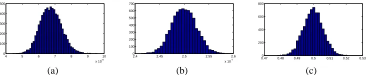
process of interest is removed efficiently. Figure 3 shows the distribution of the estimates of these parameters over the 7,500 simulated paths forθ1 = 0.5; the estimation procedure is unbiased and

The estimators_h\X, X_i(s_T1)and_h\X, X_i(m_T 1)are inconsistent when additional structure is permitted in the noise. We stress that these are estimators based on assumptions of white noise, and their strong performance in this instance (θ1 = 0) is apparent. As we move away from white noise,

\

hX, X_i(s_T1)and_h\X, X_i(m_T 1) overcompensate for the noise whenθ1in near minus one and

under-compensate whenθ1 is near one. This happens because as the value ofθ changes, taking values

between minus one and one the spectral properties of the noise process change quite markedly with the appropriate shrinkage factor changing form in a corresponding fashion. For negative values of

θ1the multiscale ratio, and smaller positive values ofθ1the augmented multiscale ratio is

decreas-ing at higher frequencies, whilst whenθ1approaches one the multiscale ratio is not monotone (see

Figures 1(c), 2(a) and 2(b))._h\X, X_i(m_T 1)seems to still perform well for negativeθ1values (note how

the spectral form of the noise process is still largely the same shape) but performs disastrously for positiveθ1values, due to the larger energy at lower frequencies that the estimator fails to remove.

\

hX, X_i(s_T1)suffers equivalent loss of performance asθ1moves away from zero in each direction;

for such a time-domain estimator to perform better in these instances, the optimal subsampling rate of the estimator would have to be re-calibrated to incorporate the correlated noise. Nevertheless, all the estimators perform better than the noise polluted and biased estimator of the quadratic variation

onYt,h\X, Xi (b) T .

5

Conclusions

This paper has proposed extending the multiscale estimation methods of Sykulski et al for inte-grated volatility to include the case of stationary high frequency nuisance structure. It was found that naively applying estimators designed for the case of uncorrelated noise did not perform well. By modelling the nuisance structure as a Moving Average process, better bias correction could be applied at each frequency, and this substantially improved our estimator of the integrated volatility. Despite greater flexibility, the performance of the estimator did not deteriorate in terms of mean square error, which could have been a possible outcome. Note that the multiscale methods did not include parametric modelling of_{Xt}only approximating its multiscale nature. Future avenues of

investigation includes rigorous model choice procedures, and the application of Bayesian estimation methods to naturally incorporate the multiscale ratio by Hierarchical modelling. Multiscale mod-elling shows great promise for designing inference methods for continuous time processes, by the increase in precision and power from investigating properties directly scale-by-scale.

References

[1] L. Zhang, P. A. Mykland, and Y. Ait-Sahalia, “A tale of two time scales: Determining inte-grated volatility with noisy high-frequency data”, J. Am. Stat. Assoc., vol. 100, pp. 1394–1411, 2005.

[2] G. A. Pavliotis and A. M. Stuart, “Parameter estimation for multiscale diffusions”, J. Stat.

Phys., vol. 127, pp. 741–781, 2007.

[3] J. Fan and Y. Wang, “Multi-scale jump and volatility analysis for high-frequency financial data”, J. of the American Statistical Association, vol. 102, pp. 1349–1362, 2007.

[4] A. Sykulski, S. C. Olhede, and G. Pavliotis, “Multiscale inference for high-frequency data”, Tech. Rep. 290, Department of Statistical Science, University College London, arxiv.org/abs/0803.0392, 2008.

[5] Heston, “A closed form solution for options with stochastic volatility with applications to bond and currency options”, Review of Financial Studies, vol. 6, pp. 327–343, 1993.

[6] M. E. Mancino and S. Sanfelici, “Robustness of fourier estimators of integrated volatility in the presence of microstructure noise”, Tech. Rep., University of Firenze, 2006.

[7] M. Lo`eve, Probability theory. I, Springer-Verlag, New York, fourth edition, 1977, Graduate Texts in Mathematics, Vol. 45.

0 0.1 0.2 0.3 0.4 0.5 0

1 2 3 4 5 6 7x 10

-8

frequency

(a)

0 0.1 0.2 0.3 0.4 0.5 0

1 2 3 4 5 6x 10

-6

frequency

(b)

0 0.1 0.2 0.3 0.4 0.5 0

0.2 0.4 0.6 0.8 1

frequency

(c)

0 0.1 0.2 0.3 0.4 0.5 0

1 2 3 4 5 6 7x 10

-8

frequency

(d)

Figure 1: (a) The periodogram of a realisation ofU_t(X)(solid line), (b) of a realisation ofU_t()(solid line) with the Whittle estimates superimposed (white solid line), (c) the estimate ofLkfrom the raw

periodograms of the unobserved processes (solid line) with the Whittle estimateLck superimposed

(white solid line) and (d) the bias corrected estimator of the periodogram ofU_t(X), usingLbk. θ1=

0.5in this example. Notice the different scales in the four figures. Estimated spectra are here plotted on a linear scale for ease of comparison to the effect of applyingLk.

0 0.1 0.2 0.3 0.4 0.5 0

0.2 0.4 0.6 0.8 1

frequency

(a)

0 0.1 0.2 0.3 0.4 0.5 0

0.2 0.4 0.6 0.8 1

frequency

(b)

Figure 2: The estimate of Lk from the raw estimated spectra of the unobserved processes (solid

line) with the Whittle estimateLck(white solid line) superimposed for (a)θ1=−0.5and (b)θ1= 1.

4 5 6 7 8 9 10 x 10-9 0

100 200 300 400 500

(a)

2.4 2.45 2.5 2.55 2.6 x 10-7 0

100 200 300 400 500 600 700

(b)

0.470 0.48 0.49 0.5 0.51 0.52 0.53 200

400 600 800

(c)

Figure 3: Histograms showing the distribution of the estimators of the parameters inLbk, for (a)σ2X,

(b)σ2

and (c)θ1(where the true value ofθ1is0.5) over 7,500 simulated paths.

[9] D. Brillinger, Time series: data analysis and theory, Society for Industrial and Applied Mathematics, Philadelphia, USA, 2001.

[10] J. Beran, Statistics for long-memory Processes, Chapman and Hall, London, 1994.

[11] K. O Dzhamparidze and A. M. Yaglom, “Spectrum parameter estimation in time series analy-sis”, in Developments in Statistics, PR Krishnaiah, Ed., vol. 4, pp. 1–181. New York: Academic Press., 1983.