19 RULE MINING FOR DYNAMIC DATABASES
A Das & D K Bhattacharyya Department of Information Technology Tezpur University, Napaam 784 028, India E-mail : [email protected], [email protected]
ABSTRACT
Association rules identify associations among data items and were introduced in 1993 by Agarwal et al.. Most of the algorithms to find association rules deal with the static databases. There are very few algorithms that deal with dynamic databases. The most classical algorithm to find association rules in dynamic database is Borders algorithm. This paper presents two modified version of the Borders algorithm called Modified Borders.
Experimental results show that the modified version performs better than the Borders algorithm in terms of execution time. To address the scalability issue, the paper also proposes a distributed version of the Borders algorithm, called Distributed Borders.
Keywords: Rule mining, itemset, frequent items, support, confidence, border sets, promoted border sets.
INTRODUCTION
Association Rule is one of the most vital areas of research in data mining and was introduced by Agarwal et. al in 1993 [Agarwal(1993)]. Association rules are of the form “80% of the customers who buy bread also buy butter". In other words association rules find the influence of one set of items on another set of items. Association rules have got numerous applications in real world such as decision support, understanding customer behavior, telecommunication alarm diagnosis and prediction, etc. The departmental stores also can use association rules in many fields such as catalog design, add-on sales, stored layout etc.
The terms most frequently used in relation to association rules are itemset, support, confidence, frequent itemsets . An itemset means a non-empty set of items. The support of an itemset X is defined as the % of transactions/records in a database that contains X. An itemset with support greater than the some pre-defined minimum support is called a
frequent or large itemset. An association rule between two disjoint and frequent itemsets X
and Y exists, if X ∪Y is frequent and confidence is at least some pre-defined value. Confidence of an association rule between X and Y is defined as the percentages of transactions/records that contain X also contain Y.
Finding frequent itemset is one important step in association rule mining. There are some influential algorithms to find the frequent itemsets from large databases. The most classical algorithm is Aprior (Agarwal(1994)). Some other important algorithms are AprioriTid
[Agarwal(1994)], FP-Tree [Han(2000)], Partition algorithm[Savasere (1995)], DIC
algorithm[Brin(1997)] etc.
20 in the updated database to find the frequent itemsets in the updated database. However, this is not the optimal solution because of the following reasons.
1. It will require running the algorithms on adding, deleting or updating a small number of records.
2. It will take too much time because it will scan the same database every time.
3. It will generate most of the itemsets repeatedly
Literature shows that there are some algorithms to find frequent itemsets in dynamic databases. Some of them are FUP [Cheung(1996)], FUP2[Cheung(1997)] ,DELI[Lee(1998)], MAAP[Ezeife(2002)]. Some more works can be found in [Thomas(1997), Feldman(1997)]. The main requirements of a dynamic association rule-mining algorithm are
1. It should be able to use the already discovered frequent itemsets to discover new frequent itemsets.
2. It should not have to scan the old records/transactions.
3. It should scan the new records/transactions as few number of times as possible.
The most popular and important algorithm, which follows the above criteria, to find frequent itemsets in dynamic database is the Borders algorithm [Feldman(1999)]. This algorithm has used the concept of border and promoted border set to update the frequent itemsets. However, the algorithm suffers from scalability problem and cannot be used in distributed environment. To address these problems, this chapter presents a modified version of Borders algorithm, which takes less time than that of Borders algorithm. This chapter also presents a Distributed Border algorithm, which is meant for distributed dynamic databases. Symbols given in Table 1 are used to explain the algorithms.
BORDERS ALGORITHM
Feldman et. al. [Feldman(1999)] proposed Borders algorithm, which uses the concept of
border set. There are three variations of Borders algorithm : addition of transactions/records; addition and deletion of transactions/records ; changing of minimum support threshold. The main characteristics of the algorithm are as follows.
Entire database is scanned only when new candidate sets are generated.
21 Table 1: Symbols
D Database
|D| Number of records/transactions in the database D. TID Transaction ID.
X ,Y Itemsets. S(X) Support of X in % Si The site I n Number of sites. α Minimum support in % β Positive real number ( < α ) Told I Old database at the site I Tnew
i
Incremental database at site I Told The old database ( ∪Told I )
T new The newly added records/transactions (∪Tnewi ) Tdel Records/transactions to be deleted.
Twhole I
Told i ∪ Tnew I Twhole The whole database
(Told∪ T new)- Tdel
Lold Set of frequent itemsets in Told (with local support) Bold Set of border itemsets in Told (with local support).
Bold/ First border set in Told Bold // Second border set in Told Bwhole
/
First border set in Twhole Bwhole// Second border set in Twhole.\\ Lwhole
i
Frequent itemsets in Twhole at the site i Lwhole Set of frequent itemsets in Twhole Bwhole Set of border itemsets in Twhole B i Promoted border itemsets at the site I B Promoted border set (∪Bi )
F i Frequent itemsets in the updated database at the site I F Frequent itemsets in the updated database (∪FI). L whole (i) x, x ∈L whole and |x| = I
B whole i
Border itemsets in T whole at the site I B(i) b ∈ B and |b|=I
Li Frequent itemset of size i
C i Candidate itemset of size i C Set of all candidates. c A candidate itemset.
S(X) y Support count of the itemset X in the database y X.sup.new i Support of X at T new I
X.sup.new Support of X at T new
X.sup i Local support of the itemset X at the site I X.sup Global support of X
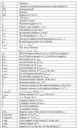
22 Figure 1 : Border Set
Actually, Manila and Toivonenn gave concept of border set. An itemset X is called a
border set if X is not frequent, but all its proper subsets are frequent. So collection of border sets forms the border line between the frequent sets and non-frequent sets. An itemset that was a border set before the database was updated and has become frequent after the database has been updated is called a promoted border set. Borders algorithm also uses the same concept and maintains support counts for all the frequent sets as well as border sets.
Input : T new , Told α, Lold and Bold
Output : Lwhole and Bwhole Scan T new and increment the support count of X ∈ Lold ∪Bold
B :={X | X ∈ Bold and S(X) Twhole ≥ α}
Lwhole := B ∪ {X | X ∈Lold and S(X) Twhole ≥ α }
B whole = {X | ∀ x ∈X,X -{x} ∈L whole } m= max {i | B(i) ≠ φ }
Candidate-generation :
L0 = φ, i =1
While( Li≠ φor i ≤ m) do
Ci+1= { X = S1∪ S2 | (i) |X|=i+1,
(ii) ∃x ∈ S1, S1 -{x}∈ B(i)∪ Li (iii) ∀ x ∈S2, S2 -{x}∈ L whole(i) ∪Li }
Scan Twhole and obtain S(X) for all X ∈Ci+1
Li+1 = { X | X ∈ Ci+1 and S(X) ≥α}
23
L whole = L whole ∪ L i+1
B whole = Bwhole ∪ Ci+1 - L i+1}
i = i+1 Enddo
Figure 2: Borders Algorithm (addition)
The algorithm is based on the observation that a set is required to be considered as a candidate set only if it has a subset that is a promoted border. The following lemma proves this observation. In addition to the lemma, the paper [Feldman(1999)] also proved that
Borders algorithm is correct.
Lemma: If X is an itemset which is frequent in Twhole and not frequent Told, then there exist
a subset Y ∈ X such that Y is promoted border.
Proof : Let Y be a minimal cardinality subset of X , which is frequent in T whole , but not in T
old. So all proper subsets of Y are frequent in T whole. However, by minimality of Y, none of
these subsets is a new frequent set in T whole. So Y is a border set in Told.
Given L old and B old, the task of the Borders algorithm is to find L whole and B whole. The
algorithm (addition) is presented in Figure 2 . The algorithm assumes that L old and Bold are known with their respective supports. L old and Bold can be found by any association rule mining algorithms like Apriori. The algorithm starts by making one pass over the new database T new and counts the supports of the itemsets of L old ∪Bold for Tnew .
During this pass the algorithm calculates B and L whole. If B is null, then L whole contains all
the frequent sets of Twhole. However, if there is at least one promoted border (i.e. B is not null), then the algorithm generates new candidate sets Ci+1 (steps 8-10 ) and scans over the
entire database to count the support of them (steps 11-13 ). Then it finds the frequent itemsets Li+1 based on the support count and updates Lwhole and B whole. This process
continues as long as new candidates can be generated. So the algorithm scans the whole database, if there is some promoted border set. Otherwise, it does not require scanning the whole database.
An example
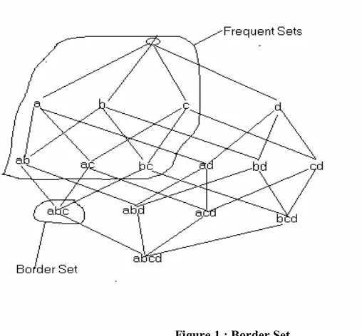
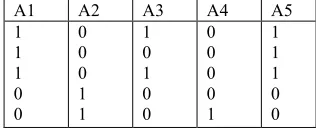
Let us take Told and Tnew as given in Table 2 and Table 3 respectively and the support be 40%.
A1 A2 A3 A4 A5
24 Table 2 : Told
A1 A2 A3 A4 A5
0 0 1 0 0 0 0 0 0 1 1 0 0 0 0 1 1 0 0 1 1 0 1 0 0 Table 3 : Tnew
Then, Lold is {(A1,A2,A3,A5), (A1A3), (A1A5), (A3A5), (A1A3A5)} and Bold is { (A4), (A1A2), (A2A3), (A2A5)}. Next, T new is added with T old. Now, T new is scanned to
calculate B, Lwhole and B whole.
B = {(A4)}
L whole = {A4 , A1 , A5, A1A5)}
B whole = {(A1A4), (A4A5), (A1A5)}
Here, we have got one promoted border (A4). So, we have to generate new candidate itemsets. New Candidates are generated in level-wise fashion as in Apriori.
Candidate 2-itemsets are C2 = { (A1A4) , (A4A5)} Candidate 3-itemsets are C3 = { (A1A4A5) }
Now the whole database T whole is to be scanned to update L whole and B whole.
Discussion :
The Borders algorithm is robust enough to find the frequent itemsets in a dynamic database. However, from our experimental study, it has been observed that
• With the increase in the volume of the Told and T new, the cost of the
scanning of T whole in the every iteration becomes too expensive. • It suffers from scalability problem.
To overcome the above problems, this paper proposes two enhanced versions of the present
Borders (addition) algorithm. These are Modified Borders and Distributed Borders.
Modified Borders has used two border sets to reduce scanning of entire database. On the other hand, Distributed Borders is the extension of Borders in distributed environment.
MODIFIED BORDERS ALGORITHM
25 will be generated only when some borders, which were not included to generate candidates in the old database, becomes promoted. Based on the above discussion, Borders has been modified by including two border sets. The first border set is Bold/ and the second border set
is Bold//. Bold/ is calculated as
{ X | ∀ x ∈X, X-{x} ∈ (L old ∪B old/ ); S(X) ≥ β and S(X) < α }. Bold// is calculated as
{X | ∀ x ∈ X, X-{x}∈ (L old ∪ B old/); S(X) < β }. Bold / and Lold take part in candidate generation, whereas the elements of Bold
//
are not used in candidate generation. Another requirement in the algorithm is that all the subsets of an itemset X ∈ (Bold/ ∪ Bold // ) must be ∈ ( Lold∪ Bold/ ). Obviously, Bold / contains the itemsets with higher probability of becoming promoted when new transactions are added. New candidate sets will be generated only when any of the elements of the Bold // becomes promoted. If new candidate itemsets are generated, one scan over the whole database is required to find supports of the new candidates.
The algorithm
The algorithm works as follows. Lold, Bold /
and Bold //
are assumed to be known with their respective support counts. The algorithm starts by making one pass over the new database
Tnew and updates supports of the elements of Lold ∪ B old /
∪ Bold //
. During the pass, the algorithm generates four categories of itemsets - B/ , B //, B/// and B //// . If B// is null, then no new candidate set is required to be generated. If B// contains at least one itemset, then new candidate sets are required to be generated. If new candidate sets are generated, the algorithm makes one pass over the entire database to count the support of the new candidate sets. At the end, the algorithm generates Lwhole, Bwhole / and Bwhole // , which are counterparts of the Lold , Bold/ and Bold // respectively, for the whole database Twhole. The algorithm is presented in the Figure 3.
Input : Tnew , Told , α, β , Lold and Bold/ , Bold//
Output : Lwhole and Bwhole/ , Bwhole //
Scan Tnew and increment the support count of X ∈ (Lold ∪Bold / ∪Bold // )
B/ = {X | X ∈Bold /
and S(X)T whole ≥ α} B// = {X | X ∈ Bold // and S(X)T whole≥ α }
Lwhole = B / ∪B// ∪ {X | X ∈ L old and S(X)T whole ≥ α }
B/// = {X | X ∈ B
old // ; ∀x ∈X, X -{x} ∈Lwhole; S(X) Twhole ≥ β and S(X)Twhole < α } B//// = {X | X∈Bold/ ∪Lold ; ∀x∈X, X -{x} ∈Lwhole ; ( S(X)Twhole ≥ β and S(X)Twhole < α
)}
Bwhole / = B /// ∪ B ////
Bwhole // = {X | ∀x ∈X, X -{x} ∈Lwhole and S(X) < β } If B // ≠ φ then
m = max {i | B// (i) ≠ φ }
Candidate-generation:
L0 = φ , B0 = φ, k=2
While (Lk-1 ≠ φ or Bk-1 ≠ φ or k ≤m+1) do Ck = φ
L = B// ( k-1) ∪Lk -1 ∪B/// (k-1) ∪B k-1
26 For all itemsets in l2 ∈ M do begin
If l1 [i] = l2[i] ( 1 ≤ i ≤k-2 ) and l1[k-1] < l2[k-1] then
C = {l1 [1], l1[2], …l1[k-2], l1[k-1], l2[k-1]}
Ck = Ck∪ C
End for
End for
Prune Ck : All the subsets of Ck of size k-1 must be present in M ;
Scan Twhole and obtain support S(X) for all X ∈Ck
Lk = {X | X ∈Ck and S(X) ≥ α}
L whole=Lwhole ∪ Lk
B k = {X |X ∈ (Ck - Lk ); ∀x ∈ X, X-{x} ∈L whole; S(X) ≥ β and S(X) < α)
Bwhole/ = Bwhole / ∪ Bk
Bwhole// = Bwhole// ∪ {X |X ∈ (Ck - Lk); ∀x ∈ X, X-{x} ∈ Lwhole ; S(X) < β ) k = k+1 ;
Enddo
Figure 3: Modified Borders Algorithm An example
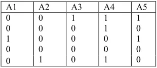
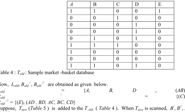
Let us consider Told as given in Table 4 and assume α = 40% and β = 30%.
A B C D E
1 1 0 0 1
0 0 1 0 0
0 0 0 1 0
0 0 0 1 0
0 1 0 1 0
1 1 1 0 0
1 0 0 0 0
0 0 0 0 0
1 1 0 1 0
Table 4 : Told : Sample market -basket database
Now, Lold, Bold /, Bold// are obtained as given below.
Lold = {A, B, D , (AB)}
Bold / = {(C)}
Bold //
= {(E), (AD , BD, AC, BC, CD}
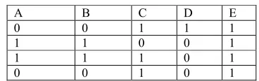
Suppose, Tnew (Table 5 ) is added to the T old ( Table 4). When Tnew is scanned, B/, B//, B ///
27
A B C D E
0 0 1 1 1
1 1 0 0 1
1 1 1 0 1
0 0 1 0 1
Table 5 : Tnew
Experimental results
We compared Modified Borders with Borders algorithm using two synthetic databases and one real database. Both the algorithms were implemented on a Intel PIV based WS (with 256 MB SDRAM). Lold, Bold , Bold
/
and Bold //
had been computed separately.
Test Data : We used synthetic databases, which were generated using the technique given in [Agarwal(1996)], and the Connect-4 dataset, which were downloaded from UCI machine learning repository(www.ics.uci.edu). All the synthetic datasets contained 100K records and dimensionality of each record is 255. Other parameters for synthetic databases are shown in the Table 6 . For all the experiments, initial sizes of the synthetic databases and
Connect-4 were taken as 80K records and 47557 records respectively.
Data Set |T| [I] |D|
T20I4100K 20 4 100K
T20I6100K 20 6 100K
Table 6 : Parameters used for synthetic data generation
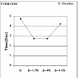
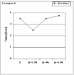
We executed each of the experiments several times. Tables 7 through 9 show average number of full database scan required in Borders and Modified Borders as the value of β increased from 3.5% to 4.5% and size of incremental database is increased from 5K records to 20K records. The value of α (minimum support) was taken as 5 % for all the experiments. Average execution times over all increments are given in Figures 4 through 6.
Table 7 : Database:T20I4100K
Table 8 : Database:T20I6100K Increment Borders Modified
(β =3.5%)
Modified
(β =4%)
Modified
( β=4.5%)
5K 1 0 0 1
10K 3 0 1 2
15K 2 0 0 2
20K 3 1 1 3
Increment Borders Modified
(β=3.5%)
Modified
(β =4%)
Modified (β=4.5%)
5K 0 0 0 0
10K 3 0 0 2
15K 2 1 1 1
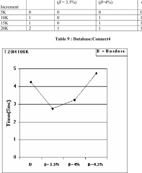
28 Table 9 : Database:Connect4
Figure 4 : Average Execution Time Increment
Borders Modified
(β= 3.5%)
Modified (β=4%)
Modified
( β=4.5%)
5K 0 0 0 0
10K 1 0 1 1
15K 1 0 1 1
30 Figure 6 : Average Execution Time
Observations
Following are some observations made from the experimental results.
• Experimental results (Tables 7, 8 & 9) show that Borders algorithm requires whole scan of the database several number of times, whereas
Modified Borders requires whole scan of database a few number of times.
• The value of β has a great effect on the performance of Modified Borders algorithm. As the value of β increases, number of whole scan also increases. In our experiments, we found that when β=4.5%, number of full scan of the database is almost same in both the algorithms.
• As far as execution time is concerned, Modified Borders takes much less time than that of Borders when β is small (Figures 4, 5 & 6 ). As the value of βincreases, Modified Borders tend to take little more time. This is because number of full scan tends to increase with the increase of value of β.
On the selection of the value of ββββ :
31 with the decrease in value of β , the memory requirement increases due to the additional candidate sets. So value of β cannot be decreased too much. This cost of additional memory requirement is quite negligible in comparison to the requirement of full database scanning, particularly when database is very large. So there should be some trade off in choosing the value of β. If there is not enough memory and the database is dense, the value of β can be set to a higher value. For sparse databases, β can be set to a lower value. Here is one simple method to adjust the value of β. For the first increment of the database, β can be set to a lower value. In the subsequent increments, β can be increased a little until number of candidates is manageable and gives desired result.
DISTRIBUTED BORDERS ALGORITHM
The Borders algorithm is sequential in nature and meant for centralized database. However, most of the databases are distributed in nature. Distributed Borders algorithm is basically meant for distributed dynamic databases. However, it can also be used in a centralized database by partitioning the database and placing the partitions in different nodes of distributed systems. This process reduces the number of candidate sets to a great extent resulting in high flexibility, scalability and low cost performance ratio [Cheung(1996),31-42]. Distributed algorithms posses some problems such as locally frequent or border sets may not be globally frequent or border sets. Again, message passing being a costly affair, processing should be confined in the local sites as much as possible. To explain the algorithm, it is assumed that databases of similar structure are distributed in different sites which are networked. Let us consider a transactional database, where each record is a transaction in a supermarket made by the customers. Each transaction is of the form <TID,1 ,1 ,0...0, 1> . Here TID is the transaction id, which is unique for each transaction. 1 and 0 represents the corresponding item has been bought and not bought respectively in the transaction. It is also assumed that the database is horizontally partitioned and allocated in n sites Si (i=1, 2, 3...n) in a distributed system. Now, the task is to maintain the global frequent itemsets and global border sets in this distributed environment when the database is updated.
Distributed algorithm for maintaining frequent itemsets in dynamic database Here, we have examined the Borders algorithm in the distributed environment. Let Told be
the old transaction database distributed in n sites. Told i is the old transaction database at the site i (i =1, 2, 3...n). Tnew and Tnew
i
are the new transactions to be added to the whole database and to the transactions at the site i respectively. X.sup and X.sup i are the global support count and local support count at the site i respectively of the itemset X. For a given minimum support threshold α , an itemset X is globally frequent in the old database(updated database) if X. sup ≥ α|Told| ( X.sup ≥α |Twhole| ). Similarly, an itemset X is locally frequent in the old database(updated database) at some site i, if X.supi
32 Given Lold and Bold, the problem here is to find updated frequent itemsets Lwhole and border sets Bwhole for the updated database Twhole.
The main purpose of the Distributed Borders algorithm is to reduce the number of candidate sets and in turn reduce the number of messages to be passed across the network and execution time. To reduce the number of messages, we used polling technique as discussed in DMA [Cheung(1996,911-921)]. Some interesting observations, which are listed below, can be made relating to frequent, border and promoted border sets in large database in distributed environment. Some of these observations were discussed in [Cheung(1996,911-921)].
1. Every global frequent itemset X must be frequent in at least one site Si. 2. If an itemset X is locally frequent at some site Si, than all its subsets are also
locally frequent in the site Si.
3. If an itemset X is globally frequent at some site S i, then all its subsets are also globally frequent at the site Si.
4. If an itemset X is globally frequent or promoted border, then X must be frequent in at least one site i.
Proof: This is obvious because if an itemset X is small in all the sites, it cannot be frequent in the whole database.
5. If an itemset X is a global promoted border set, then X must be frequent in
Tnew i for some site Si.
Proof: Let an itemset X is a promoted border set in the updated database
Twhole. Then S(X) < α |Told | and S(X) ≥α |Twhole|. Since Twhole = Told ∪Tnew ,
S(X)≥α |Tnew|. Therefore S(X) ≥α ∑ |Tnewi.| . Hence, S(X) ≥α |Tnew i| for at least one site Si.
6. If X is global border set, then there exist a Y ⊂ X so that Y is local border in some site Si.
Proof: If X is a global border set, then X must be small/infrequent in at least one site Si. Therefore, there exist at least one subset of X, which is a local border set in the site.
7. If a new candidate set c∈Twhole has to be frequent or border in Twhole , then either c or one of its immediate proper subsets must be locally frequent in one
Tnewi.
Proof : If c is a new candidate set there can be two possible cases:
a) c is frequent in the updated database Twhole : In this case c must be
frequent in Tnew i.e. c must be frequent in Tnewi for some i.
b) c is a border set in the updated database Twhole : In this case c
will be small and all of its subsets will be frequent in the updated database Twhole. So there exists at least one c / ⊂ c, which was small in the old database Told. Otherwise, c would have been
generated in the old database Told. This c / will be frequent in the updated database Twhole. So c/ must be frequent in the Tnew i.e. c /
must be frequent in Tnewi for some i.
8. If a candidate set X in the updated database is either frequent or border set, all of its immediate proper subsets must be either ∈ (F ∪ B) or frequent in at least one site.
Proof: There can be two possible cases:
33 Then, Y is either a candidate set or Y ∈F ∪ B . If Y is a candidate and Y
is frequent, then Y must be frequent in at least one site because Y
cannot be frequent if it is small in all the sites.
b) X is border in the updated database: In this case, all the subsets of X must be frequent in the updated database. So, by first option, all the subsets are either ∈ ( F ∪B ) or frequent in at least one site.
Local pruning
Using the above observations many unnecessary candidates can be pruned locally. If an itemset X is locally small in all the sites, then X cannot be frequent globally. That is why, itemsets are first checked if they are locally frequent or not. Their global support are found only when they are locally frequent in at least one site Si. Similarly some promoted border sets also can be pruned away locally using Observation 4. So, if a border set X is not frequent in any site, then it is not tested for global promoted border. Observation 7 is also very significant in pruning away candidate sets locally. After the candidate sets are generated, support of the candidate sets are counted in the incremental part Tnewi. If any
candidate set or at least one of its immediate proper subsets is not frequent in at least one
Tnewi, it can be pruned away because by Observation 7 it can be neither frequent nor border. Observation 8 is also helpful in pruning away unnecessary candidate sets.
Input: Lold , Bold, Tnewi, Told i and α
Output: Updated Lwhole and Bwhole
Repeat the following steps at each site i distributively.
Scan Tnew i and count the support of all the itemsets X ∈( Lold ∪ Bold ) and find
B i = {X|X ∈Bold and S(X)T newi ≥α | Tnewi | }
Lwhole i = B i∪ { X | X ∈Lold and S(X)Twhole i ≥α |Twhole i | } (by observation 4)
Broadcast X ∈ Lwholei to other sites along with their supports.
Prune Lwhole i : Lwhole i = { X | X ∈ Lwholei and S(X)Twhole ≥α |Twhole| } Compute B = ∪Bi and Lwhole = ∪Lwhole
i
Bwhole = {X | ∀ x ∈X, X-{x} ∈Lwhole }
Generate candidates:
m = max { i | B(i) ≠ φ }
i=1
While (Li ≠ φ or i ≤m) do
Ci+1 = { X = S1 ∪ S2 | (i) |X|=i+1,
(ii) ∃ x ∈S1, S1- {x} ∈B(i) ∪Li , (iii) ∀x ∈ S2, S2-{x} ∈ L whole (i) ∪Li }
Scan Tnew i and compute X.sup.newi for all X ∈Ci+1.
Remove any candidate set X ∈ Ci+1, which is or at least one of its immediate
proper subsets is not frequent in Tnew i (by observation 7).
Scan Told i and find the support X.sup i for all X ∈Ci+1 ( Tnew i has already been scanned)
34 observation 8)
Find the global support for all X∈Ci+1 as X.sup = ∑X.sup i
Li+1 = {X | X ∈ Ci+1 and X.sup ≥α } Lwhole = Lwhole∪ Li+1
Bwhole = Bwhole ∪ (Ci+1 - Li+1)
i=i+1 Enddo
Return Lwhole and Bwhole
Figure 7 : : Distributed Borders Algorithm Explanation of the algorithm
It is assumed that the Lold and Bold are available with the local support to all the sites. The algorithm starts with scanning the incremental portion Tnew
i
and finds local support for all X ∈Lold ∪Bold. This is because frequent sets and border sets, which are frequent locally in at least one site, can only be frequent globally. Then comes the step 2, which finds the global support for Lwholei This can be done by simply broadcasting the local support of X ∈ L wholei. If all the items are broadcast to all the sites, then for each item X, O(n2) messages will be required, where n is the number of sites. So polling techniques as described in [Cheung(1996,31-42)] can be used. This technique reduces the number of messages to O(n) for each itemset. Step 3 prunes away all X ∈ Lwhole i, which are not globally frequent. Then the Step 4 just broadcasts the Lwhole i to other sites and receives the same from other
sites to compute Lwhole and B. It can be noted that, all the sites will be having the same set of Lwhole and B. Steps 6-11 are responsible for generating the candidate sets. The
candidate sets are generated in the step-wise method like Apriori. Some kind of pruning techniques are required to prune away some unnecessary candidate sets. Observation 4
helps prune away some candidate sets. Steps 13-15 are basically pruning steps. It scans the Tnew i and finds the X.sup.new i for all the candidate sets. According to Observation 4, a candidate X can be neither frequent nor border, if neither X is frequent nor at least one of its immediate proper subsets is frequent in any Tnew i. So the candidates, which do not conform to Observation 4, can easily be removed from the candidate sets. Step 16 finds the global support for all the candidate sets. Polling technique as given in [Cheung(1996)] can be used here also. Steps 17-19 find frequent itemsets and border sets for the updated database. Finally, step 22 returns the global frequent itemsets and global border sets.
Experimental results
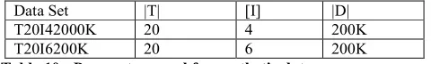
We simulated the algorithm on a share-nothing environment. A 10/100 Mb LAN was used to connect six PIII machines running Windows NT. Each machine had 20GB disk space and 256MB memory. The dataset used in the experiments were T20I4200K and T20I6200K, which were generated using the technique given in [Agarwal(1996)]. Each datasets contained 200K tuples (transactions). Each dataset was partitioned and corresponding partitions were loaded in the machines before the experiments started.
Data Set |T| [I] |D|
T20I42000K 20 4 200K
T20I6200K 20 6 200K
35 We carried out three experiments. In the first experiment, we used three machines (sites). The purpose of the experiment was to find the execution time and number of candidate sets for different minimum support. Each machine initially contained 63K transactions and 3K transactions were added to each machine as incremental database. The results are given in
Figure 8.
The second experiment was the scale up experiment. The testbed of the second experiment was same as that of first experiment. Here also we used three machines(sites). The purpose of the second experiment was to find the effect of the database size on the execution time. Three machines initially contained 30%, 30% and 25% transactions respectively. Size of incremental database was 5% for each of the machines and minimum support was 1%. The results are given in Figure 9.
The third experiment was the speedup experiment. The speedup factor is defined as
S(n)=T(1)/T(n) and efficiency is defined as S(n)/n, where T(n) is the execution time with n
sites. Here, we increased the number of machines(sites) from 1 to 6. Sizes of initial database and incremental database were taken as 80% and 20% respectively. Initial and incremental database were divided equally among the machines and minimum support was taken as 1% . When we used 1 machine(site), it was the sequential run time of the Borders
algorithm. The results are given in Figure 10.
DISCUSSION
The result of the first experiment was obvious and straightforward. In some cases execution time did not decrease significantly with the increase of minimum support. This was because whole scan of the database might be required in some sites. It was evident from the second experiment that execution time increased with the increase of the size of initial database and incremental database. . However, it increased linearly. Third experiment measured
speedup and efficiency of the algorithm. We found average efficiency of 63% and 67% for T20I6200K and T20I4200K respectively, which showed that the algorithm achieved sub-linear speedup. However, as with other distributed algorithms, performance of this algorithm also depends on the factors such as database types, distribution of data, skewness of data, network speed and other network related problems.
CONCLUSION
38 Figure 10 : Execution Time for Different Number of Sites
REFERENCES:
Agarwal R, Imielinski T and Swami A(1993) “Mining Association Rules between Sets of Items in Large Databases”, ACM SIGMOD International Conference on Management of Data, May.
Agarwal R and Shrikant R (1994) “Fast Algorithms for Mining Association Rules in Large Databases", Proceedings of 20th International Conference on Very Large Databases , August-September , Santiago, Chile,
Agarwal R, Mannila H, Shrikant R, Toivonen H and Verkamo A I(1996). Fast Discovery of Association Rules. MIT Press.
Brin S, Motwani R, Tsur D and Ullman J(1997), “Dynamic Itemset Counting and Implication Rules for Market- Basket Data", Proceedings of 1997 SIGMOD , Montreal, Canada, June.
Cheung D W, Han J, Vincent T Ng, W Fu Ada, and Fu Y(1996) “A Fast Distributed Algorithm for Mining Association Rules”, Proceedings of 4th Inernational Conference on Parallel and Distributed Information Systems , pages 31–42. Cheung D W, Ng V T, Ada W Fu and Fu Y(1996) “Efficient Mining of Association Rules
in Distributed Databases”, IEEE Transactions on Knowledge and Data Engineering , December , 911-921.
39 International Conference on Data Engineering, New Orleans, Louisiana.
Cheung D W, Lee D W, and Kao S D(1997). “A General Incremental Technique for Maintaining Discovered Association Rules”, In Proceedings of the fifth International Conference on Database System for Advanced Applications, Melbourn, Australia. Ezeife C I and Y Su(2002). “Mining Incremental Association Rules with Generalized FP
Tree”, Proceedings of 15th Canadian Conference on Artificial Intelligence, AI2002, Calgary, Canada, May.
Feldman R, Aumann Y, Amir Y, and Mannila H(1997) “Efficient Algorithms For Discovering Frequent Sets in Incremental Databases” , Proceedings of ACM SIGMOD Workshop on Research Issues on Data Mining and Knowledge Discovery(DMKD).
Feldman R, Aumann Y and Lipshtat O(1999) “Borders : An Efficient Algorithm for Association Generation in Dynamic Databases” , Journal of Intelligent Information System, pages 61–73.
Han J, Pei J and Yin Y (2000) “Mining Frequent Patterns without Candidate Generation”, Proceedings of the 2000 ACM-SIGMOD International Conference on
Management of Data, Dallas, Texas, USA.
Lee S D, Cheung D W and Kao B(1998). “Is Sampling Useful in Data Mining? A Case in The Maintenance of Discovered Association Rules”, Data mining and Knowledge Discovery.
Savasere , Omiecinski E and Navathe S (1995), “An Efficient Algorithm For Mining Association Rules in Large Databases”, Proceedings of 21st Conference on Very Large Databases, Zurich, September.