Small price change response to a large devaluation in a menu cost model

Munich Personal RePEc Archive

Small price change response to a large

devaluation in a menu cost model

Bruchez, Pierre-Alain

3 April 2007

Online at

https://mpra.ub.uni-muenchen.de/3541/

Small Price Change Response to a Large

Devaluation in a Menu Cost Model

Pierre-Alain Bruchez

3 April 2007

I would like to thank my thesis advisor Professor Philippe Bacchetta for useful com-ments, as well as, along with Olivier Jeanne, for getting me launched in this research direction. I would also like to thank the members of my thesis committee: Professors Harris Dellas, Jean Imbs and Giovanni Favara.

y_{Mailing address: Gesellschaftsstrasse 79, 3012, Bern, Switzerland.}

Small Price Change Response to a Large

Devaluation in a Menu Cost Model

Abstract

In an empirical paper based on …ve large devaluation episodes in

Ar-gentina, Brazil, Korea, Mexico and Thailand, Burstein and al. (2005a) …nd

a very slow adjustment in the prices of non-tradable goods and services

af-ter large devaluations. Burnstein and al. (2005b) develop a quantitative

general-equilibrium model that can account for this phenomenon. I consider

an alternative, simpler model and explore under which conditions moderate

menu costs can explain the muted response of the prices of non-tradables.

The key new element in this alternative model is a nominal friction in

wage-setting (generated by menu costs for changing wages). I …nd, for example,

that although my model is based on menu costs, it is able to deliver not only

constant prices of non-tradables, but also small price changes (in reality these

prices do change, albeit by far less than the exchange rate). I also discuss

the existence of multiple equilibria and the role of central-bank credibility.

Keywords: large devaluation, exchange rate, pass-through, sticky prices,

1

Introduction

In an empirical paper based on …ve large devaluation episodes in Argentina,

Brazil, Korea, Mexico and Thailand, Burstein and al. (2005a) …nd a very

slow adjustment in the prices of non-tradable goods and services to large

de-valuations. Burnstein and al. (2005b), henceforth BER, address the question

of why the rate of in‡ation for non-tradable goods is so much lower than the

rate of devaluation. They develop a quantitative general-equilibrium model

that can account for this phenomenon. They assume menu costs for changing

a price and show that producers of non-tradables might prefer not to change

their price at all even if the devaluation is large. There are also cases in

which it is not sustainable as an equilibrium phenomenon for …rms in the

non-tradables sector not to change their prices at all (in these cases it is

argued that real shocks are the primary driver of real exchange-rate

move-ments). They incorporate several assumptions into their model that mute

the response of the price of non-tradables to the exchange-rate shock. First,

the share of tradable goods in the consumer price index (CPI) is small.

Sec-ond, there are domestic distribution costs associated with the sale of traded

goods. Third, there is a low elasticity of the demand for exports. Fourth,

non-tradables.1 _{Moreover, they deviate from the Dixit-Stiglitz model, adopting}

Kimball’s (1995) assumption that the elasticity of demand for the output

of a monopolistic producer is increasing in its price relative to the prices of

its competitors’ goods. They conclude, however, by noting a shortcoming of

their paper: the price of non-tradables does not change at all, while in reality

these prices do change, albeit by far less than the exchange rate.2

Like BER, I aim at explaining why the rate of in‡ation for non-tradable

1_{The price of tradables will change after an exchange-rate shock. The direct impact of}

this price change on non-tradables will, however, be small since BER assume a moderate elasticity of substitution between tradables and non-tradables. But even if this elasticity were zero, there would still be other channels through which price adjusments could be induced. For example households would ask for higher wages in order to mute the impact of the increase of the prices of tradables on their real wages. This would incite …rms to increase their prices in order to pass the price increase of the labor input on to consumers. However, incorporating several assumptions that mute responses allow BER to get sticky prices with moderate menu-costs.

2_{BER focus on rationalizing an equilibrium in which non-tradable goods prices do not}

goods is so much lower than the rate of devaluation. I consider an

alter-native, simpler model and explore under which conditions moderate menu

costs can explain the muted response of the prices of non-tradables. The key

new element in this alternative model is a nominal friction in wage-setting

(generated by menu costs for changing wages).3 _{For tractability, I consider a}

partial-equilibrium model rather than a general-equilibrium model like that

of BER.

The intuition as to why this may explain small (but possibly not zero)

changes in the prices of non-tradables is the following. In a setting in which

the markup is a constant proportion of the marginal cost, the desired price

varies in the same proportion as the marginal cost. The marginal cost can

vary through two channels: a productivity change (due to a change in the

quantity produced if returns to scale are not constant) or a change in the

prices of production factors. A devaluation increases the price of imported

goods and tends to move consumption toward non-tradables, thus increasing

the quantity of non-tradables produced and reducing marginal productivity

(assuming decreasing economies of scale). Since I use the moderate elasticity

3_{I owe the idea of introducing wage stickiness, and, more generally, the model I use}

of substitution between tradables and non-tradables assumed by BER, this

…rst channel by itself motivates a price change, albeit by far less than the

exchange rate. This leaves the second channel: the wage (I assume that labor

is the only production factor). If workers do not want to reset their wage, this

second channel is not active. Then the desired price change of non-tradables

…rms is small, and this small change will occur if their menu cost is small

enough. But why would workers not reset their wage after a large devaluation

although they have two incentives to do so: i) to preserve their real wage and

ii) to compensate for higher labor disutility due to the increased quantity of

labor they must furnish? These two incentives may be so weak that they do

not outweigh even a moderate menu cost of resetting wages. First, the change

in price level is moderate since the change of the price of non-tradables is

small and the share of pure tradables (exclusive of distribution costs) in the

CPI is assumed, as in BER, to be moderate. Second, the change of labor

is also moderate since, as discussed above, production of non-tradables does

not increase much (and the production of tradables doesn’t change much

either, since the prices of tradables are assumed to adjust completely and

there is no substitution between domestic and foreign tradables4_).

exoge-I will try to avoid the shortcoming of BER consisting in not explaining

small positive changes in the prices of non-tradables. The di¤erence between

a small price response and no price response may seem to be irrelevant. It

is not. A small di¤erence may matter a great deal if it casts doubt upon

the underlying theory. In our case, one could think that a simple

menu-cost model can explain that prices do not change at all, if the menu menu-cost

is high enough, but would not be able to explain (without an exogenous

price-staggering process) why prices adjust only partially. If a …rm pays the

menu cost, why would it not adjust fully? This paper shows that a

menu-cost model can explain partial adjustment. In another setting, the same

concern has been expressed, for example, by Midrigan (2006) (he proposes

an extension of the state-dependent model in order to explain small price

changes and other micro-economic facts): “The large number of small price

changes observed in the micro-price data might lead one to conclude against

state-dependent pricing models.”

Assuming staggered price setting (like the Calvo process) and strategic

complementarity in price setting is the standard way to generate partial

ad-justment. However, assuming a time-dependent process is particularly

able after a large shock. Moreover, whereas the Calvo process is motivated

by menu costs, these menu costs do not appear explicitly. Since I want to

examine how high these menu costs need to be to explain incomplete price

adjustment after a large devaluation, I need to explicitly have these costs in

the model.

For realistic values of the parameters, I get strategic complementarity

in price and wage setting. If all …rms and workers adjust their prices and

wages, then any agent choosing to deviate would bear a large cost. Thus,

the equilibrium at which all agents adjust always exists for realistic menu

cost values. There may however also be other equilibria. If no agent adjusts,

then no agent would gain much by adjusting. Since this gain can be wiped

out by a small menu cost, no adjustment will also be an equilibrium as long

as the menu cost is not too small.

Interestingly, there are still other equilibria. In particular, workers may

prefer not to change their wages at all after a transitory devaluation. In

this case, …rms in the non-tradables sector will not choose to fully adjust

their prices to the devaluation. I compute the minimal menu cost for wages

increases by a small amount. The existence of this equilibrium, and more

generally the discussion of multiple equilibria, are the main contributions

of this paper, whereas BER focus on rationalizing an equilibrium in which

non-tradable goods’ prices do not change at all. At the core of my paper are

…gures that make it possible to understand how the set of multiple equilibria

depends on values of menu costs.

I also discuss the role of central-bank credibility. A credible central bank

can eliminate the equilibrium in which all agents adjust. If the central bank

is not credible, it will have to generate a recession to achieve this result.

The plan of this paper is as follows. The assumptions of the model are

presented in section 2. Section 3 presents the equilibrium equations. Section

4 shows that small menu costs are enough to prevent a large change in the

non-tradables price and that it is possible for the prices of non-tradables to

change by a small amount. Section 5 shows that wage rigidity plays a crucial

role in getting this result. Section 6 discusses the importance of central-bank

2

Assumptions of the model

This is a small open economy model. Non-tradables are produced with labor,

and there is a domestic endowment of tradables. The non-tradable goods

market, as well as the labor market, are cleared. Producers of non-tradables

are price setters and households are wage setters. The timing is as follows:

…rms and households predetermine nominal prices before the occurrence of a

devaluation shock. First, domestic producers set their prices and households

set their nominal wages. Then the state of the world (devaluation or

no-devaluation) is revealed, and price and wage setters decide to maintain prices

and wages at the preset levels, or to pay the menu cost and change them in

response to the shock.

Firms maximize pro…t. There are two sectors: the tradables and the

non-tradables sectors. There is a continuum of di¤erentiated non-tradable

goods produced by a mass 1 of monopolistic producers i 2 [0;1] with the

production function yi =ANLi.

The country exports or imports a tradable good (balanced trade account

is not assumed) for which the law of one price applies. Normalizing the dollar

to the exchange rate S:

PT =S .

For simplicity’s sake, the country is assumed to receive an exogenous

endowment of tradable goods.

There is a continuum of mass 1 of atomistic households indexed by h.

Each household provides its particular brand of labor, and the labor used in

production is a CES composite of the di¤erent brands given by

Li =

Z

l 1

h;i

1

; >1 ,

wherelh;i is the amount of labor provided by householdhto …rmi. The total

amount of this labor composite in this economy is given by L=

1

Z

0

Lidi.

Households maximize the following utility

uh =ch

l_h1+

1 +

under the budget constraintchP =whlh, whereP = PT1 + (1 )P

1

N

1 1

is the general price level, wh is the wage received by householdh, and ch is

a CES index of the consumption of tradable and non-tradable goods

C = 1C 1

T + (1 )

1 C

1

N

1

Notice that pro…t revenues are not included in the budget constraint.

This will simplify the expression for the household’s opportunity cost of not

adjusting its wage after an exchange-rate shock. This assumes that workers

have only labor income, while non-tradables producers earn pro…ts but no

labor income and do not consume any non-tradables.

The consumption of non-tradable goods is itself a CES composite of

dif-ferent varieties:

CN =

Z

C 1

N;i di

1

; >1 .

The structure of nominal stickiness is as follows. In the non-tradables

sector, nominal prices are set before the occurrence of the shock, and can be

changed after this occurrence at a certain cost to the price-setter (all …rms

have the same menu cost): if a …rm chooses to adjust its prices, then menu

costs are subtracted from its pro…ts. Prices can be changed at no cost the

next period. This is the same assumption, as for example, in Fishman and

Simhon (2005). Their interpretation is that …rms receive new inventories in

odd-numbered periods, at which time labels must be applied to newly-arrived

units. Therefore, in an even-numbered period, changing a unit’s price relative

to the preceding period involves the additional cost of changing labels; in

a price change is costless. Thus, prices are assumed to be sticky for at most

one period. In the same way, wages are set by the households for one period

before the occurrence of the shock and can be changed after this occurrence

at a certain cost (the same menu cost for all households): if a household

chooses to adjust its wages, then menu costs are subtracted from its utility.

Alternatively, the exchange-rate shock can be assumed to be transitory and

to last (and be expected to last) only one period.

After prices have been set, the economy can be in one of two states

char-acterized by di¤erent nominal demands and exchange rates. The state of

no-devaluation occurs with a probability that, for simplicity’s sake, is

as-sumed to be very small, so that the dependence of the preset levels on what

would happen in case of a shock can be disregarded although anticipations are

rational. In the no-devaluation state, the exchange rate is given by S =Sf

and domestic nominal demand is given by PN;fCN;f +PT;fCT;f = Nf. In

the devaluation state this becomes S = Sd and PN;dCN;d +PT;dCT;d = Nd,

where Sd Sf

Sf is the rate of devaluation. Nf and Nd are exogenous. Notice

that PNCN +PTCT = N can also be written C P = N. There are two

ways to interpret the exogeneity of N. First, one could assume that a

real money balances: C = M

P , whereM is the nominal money stock. ThenN

is simply equal to M chosen by the central bank.5 A second interpretation

of the exogeneity of N is that it is a way to capture other shocks.

What-ever the interpretation, C is given by N

P whereN is exogenously given. This

exogeneity explains why the impact on demand of interests paid or received

from the rest of the world need not be considered.

3

Equilibrium equations

The equilibria are given by the six following equations. Each variable in

this system of equations is a ratio of the corresponding variable in case of a

shock to this variable in the absence of a shock (labelled by the name of the

corresponding variable with an index "r").6

5_{The choice ofM would also have an impact on the exchange rate. If we want to keep}

the exchange rate shock exogenous in this interpretation, we need to assume that there is a (transitory) disconnect between the exchange rate andM.

6_w

r for wages,Pr for the price level, PN r for the price of the non-tradable aggregate,

Cr = N_Pr

r for the CES index of the consumption of tradable and non-tradable goods,Nr

3.1

Optimization by …rms in the non-tradables sector

Since the probability of a devaluation is assumed to be very small, the

pre-set price can be considered equal to the price that would maximize pro…ts in

the absence of a shock. Assuming that the …rm is committed to satisfying

any demand at the chosen price, pro…ts in cases of price adjustment a

(menu costs not yet subtracted) and without price adjustment n can be

computed. The di¤erence between a and n yields the …rm’s private cost

of not adjusting (as it is well known, the social cost is higher because of

externalities) during the sole relevant period (by assumption the impact of

the shock is transitory). To get a sense of its magnitude, it is useful to take

the ratio of this di¤erence to pro…t in the absence of a shock. This yields:

a n

= (wr)

( 1)

[1 (1 1 ) ] Z

1

[1 (1 1 ) ]

1 1 1

1

Z wrZ

1

1 1 ,

(1)

whereZ = (PN r) (Pr) Cr andCr = 1(except for section 6, real

consump-tion will be assumed, for simplicity’s sake, to be constant).

If GN is the cumulative of non-tradables …rms’ menu costs (expressed

adjust their prices is given by N = GN a n . Since GN is assumed to

be degenerated (all …rms have the same menu cost), N is either 0 or 1

depending on whether a n _{is smaller or larger than the common menu}

cost ( N may take an intermediate value in the special case when a n is

exactly equal to the common menu-cost, since some …rms may adjust while

other …rms do not).

3.2

Optimization by households

Similarly, the ratio of the household’s utility cost of not adjusting (Ua Un)

to its utility in the absence of a shock (U) can be computed, whereUa is the

utility in case of wage adjustment (menu costs not yet subtracted) and Un is

the utility if the household does not adjust its wage. This household’s private

cost of not adjusting its wage during the sole relevant period (expressed as a

proportion of its utility in the absence of a shock) is:

Ua Un

U = Pr Lrwr 1+

1+ ₁ 1

1

1 +

! 1"

Pr 1Lrwr (Lrwr)

1+ 1

1

1 +

#

.

(2)

pro-portion of U), then the proportion w of households that adjust their wages

is given by w = Gw Ua_UUn . Again, the cumulative is assumed to be

de-generate (all households have the same menu cost).

3.3

De…nitions and market clearing conditions

The aggregate wage level is given by w =

2

4

1

Z

0

(wh)1 dh

3

5

1 1

where wh is

the wage set by household h. Knowing that a proportion w of households

adjust their wages, and knowing which proportion of adjusting households

will change their wages, wr can be computed:

wr = w

h

Pr(Lr) (wr)

i 1 1+

+ (1 w)

1 1

. (3)

A similar computation can be made for the aggregate price for

non-tradables, the aggregate price level and aggregate labor:

PN r =

(

N

h

(wr) (Pr) (1 )(Cr)1 (PN r)( )(1 )i

1

[1 (1 1 ) ] + (1

N)

) 1 1

,

(4)

Pr =

"

(PT r)1 + (PN r)1 + 1

# 1 1

where = PTCT

PNCN ,

Lr = N (wr) (PN r) (Pr) Cr

1

[1 (1 1 ) ] +(1

N) (PN r) (Pr) Cr

1 .

(6)

4

Cases when wages are not adjusted

A change in the price of tradables has an impact on the price of non-tradables

through the goods market (if 6= 0) and through wages (I assumeCr

exoge-nous and equal to 1). If households’ menu costs are high enough for wages

to stay constant (and thus wr = 1), then there is only the goods market

channel left, through which the impact might not be strong if the elasticity

of substitution is close enough to 0 (BER set = 0:4)7_.

Formally, equation (4) becomes:

(PN r)1 = N

8 < : " PT r PNr 1 +1 +1

# (1 ) 1

(PN r) (1 )

9 =

;

1

[1 (1 1 ) ]

+ (1 N),

where N is given by equation (1).

7_{Intuitively, if w}

r= 1and = 0, then we should have PN r = 1since there is no open

channel left. Formally, equation (4) becomes in this case: PN r1 = NP

(1 ) 1

1 +

N r +1 N

If the menu costs of …rms are su¢ciently high, thenPN r = 1. This

hap-pens if their menu costs are higher than their private costs of not

adjust-ing their prices, which is equal (accordadjust-ing to §3.1) to the followadjust-ing

criti-cal value: Z 1

[1 (1 1 ) ] h

1 1 1 i 1h_{Z Z}1 ₁ 1 i_where

Z = (Pr) and Pr =

h

(PT r)1 +1

+1

i 1 1

. The assumption that wages are

not adjusted implies (according to §3.2) that households’ menu costs are

larger than (Pr) Lr

1+

1+ ₁ 1

1

1+ 1

(Pr) 1Lr (Lr)1+ 1

1

1+

where Lr = (Pr) and Pr =

h

(PT r)1 +1

+1

i 1 1

.

If non-tradables …rms have small enough menu costs then they will

change their prices. Then N = 1 (I assume that …rms’ menu costs are

strictly smaller than the critical value and do not discuss the case in

which they are exactly equal to the critical value). Equation (4)

be-comes: (PN r)1

1

( + 1) = PT r

PN r

1

+ 1. This implicit equation

forPN r has only one solution. KnowingPN r andwr, critical menu costs

Numerical example

Let’s numerically evaluatePN r and the critical menu costs for the

follow-ing calibration:

Value Justi…cation

= 0:4 BER. They quote Stockman and Tesar (1995), Lorenzo, Aboal and

Osimani (2003), and Gonzales-Rozada and Neumeyer (2003).

= 0:25 BER. This value implies a labor-supply elasticity that coincides with

the standard value used in the real business-cycle literature.

= 1=3 Implies that the pre-devaluation share of tradable goods in CPI

(distribution costs not included) is 25%. Burnstein et al. (2005a)

argue that tradable goods (distribution costs included) account for

roughly 50% of the CPI basket, but that about half of their costs

are distribution costs. This leaves a share of 25% for pure

tradable goods.

= 6 This is a benchmark in the literature.

= 2 Naknoi (2005) referring to the study by Huang and Liu (2002) who

…nd that it can vary from 2 to 4.

= 2=3 Is a realistic value for the share of labor income in GDP.

Cr = 1 Real consumption is assumed not to be a¤ected by the devaluation.

PT r = 2 The devaluation shock is such that the domestic currency loses

half of its value and the price of tradables doubles.

not change their prices if their menu costs are larger than2:4 10 3_{. In this}

case, households’ menu costs must be larger than 2:8 10 2 _{for households}

not to change their wages. If non-tradables …rms have menu costs small

enough to change their prices, then they adjust their prices by a factorPN r =

1:04. The critical …rms’ menu cost, below which they adjust their prices, is

4:3 10 2_{. This critical value is larger than the critical value obtained}

in the case that other non-tradables …rms do not adjust (2:4 10 3_{) since}

adjustment of other non-tradables prices create an extra incentive for a given

non-tradables …rm to adjust its price. This means that for a menu cost

between 2:4 10 3 _{and 4:3 10} 2 _{a non-tradables …rm will adjust its price}

or not depending on whether other …rms do or not (multiple equilibria). The

menu cost of households has to be larger than 3:3 10 2 _{for them not to}

increase their wage although the prices of non-tradables have increased.

For this calibration, this numerical example shows that a low small …rms’

menu cost is enough to be consistent with non-tradables …rms not changing

their prices. Since the price of non-tradables does not change, a quite low

households’ menu cost is enough for households not changing their wage to

be an equilibrium. Moreover, I also obtain the possibility that the price

obtained in the BER model).

5

Cases when wages are adjusted

Let’s assume now that households’ menu costs are small enough for all wages

to adjust. Then equation (3) yieldswr=Pr(Lr) where the amount of labor

depends, according to (6), on the quantities the …rms want to produce, and

thus on the prices they set.

If non-tradables …rms have large enough menu costs to prevent them

from adjusting their prices, then PN r = 1, Lr = (Pr) , wr = (Pr)1+

and the critical menu costs under which these results yield can be

computed.

Non-tradables …rms will adjust if they have small enough menu costs.

In this case equations (3) and (4) yield(PN r) + (1 )= (wr) (Pr) (1 )

and wr = Pr (wr) (PN r) (Pr) [

1 (1 1 ) ]

. Plugging equation (5)

for Pr into these equations yields two curves in the plane< PN r;wr >.

The solution is the intersection. Then knowingPN r andwr, the critical

For the above calibration I get the following values. A non-tradables …rm

will not adjust its price when other non-tradables …rms do not adjust if its

menu cost is larger than 0:11. This critical value is higher than what it was

when households did not adjust their wages since wage adjustment creates

an additional incentive for …rms to adjust their prices (households multiply

their wages by a factor1:3which is smaller than the exchange-rate shock but

is still large enough to create a big incentive for …rms to change their prices).

This critical value is so large that in this model it is very unlikely that a

…rm will not adjust its price while the households are adjusting their wages.

This is the case even when the other non-tradables …rms do not adjust their

prices. If they do, then the incentive to join them is even greater. I …nd that

for any realistic menu-cost values, an agent will always adjust when all the

other agents (households and non-tradables …rms) do, and in this case price

and wage adjustments are complete. Thus, for this calibration I do not get

sticky prices for low …rms’ menu costs if households’ menu costs are small

enough for them to change their wages. Wage stickiness was crucial to get

the results of the previous section.

The equilibria discussed in this and in the preceding section are shown as

below, other equilibria exist but they are unstable).

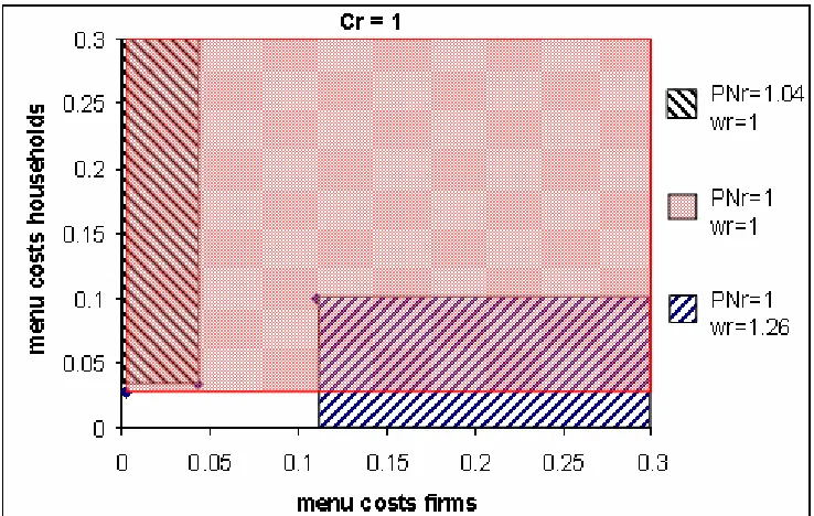
Figure 1: Stable equilibria as a function of menu costs for Cr = 1

= 0:4, = 0:25, = 1=3, = 6, = 2, = 2=3, Cr = 1,PT r = 2.

This …gure shows that full adjustment is an equilibrium for all realistic

values of menu costs. If menu costs are su¢ciently small, this is the only

equilibrium. However, there are multiple equilibria for some larger menu

costs. For these parameter values, the equilibrium (hatched slanting to the

adjust while the wages adjust, exists only for unrealistically high …rms’ menu

costs. But it is possible that neither the prices of non-tradables nor wages

adjust (shaded area). It is also possible that wages do not adjust while prices

do adjust (hatched slanting to the left).

This …gure gives the equilibria as a function of …rms’ and households’

menu costs. A …gure showing the equilibria in the plane < PN r;wr > can

also be drawn. If the menu cost of …rms is 2% and the menu cost of households

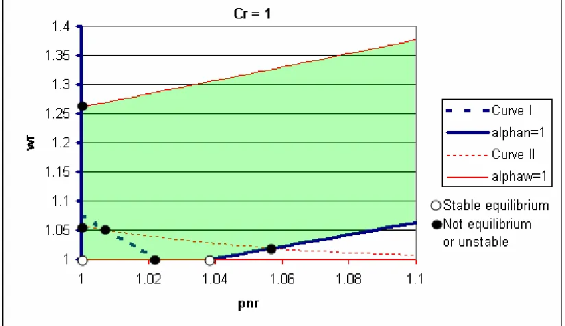
Figure 2: Potential equilibria (zoom) for Cr= 1

= 0:4, = 0:25, = 1=3, = 6, = 2, = 2=3, Cr = 1,PT r = 2,

…rms’ menu costs= 2%, households’ menu costs = 4%.

In this …gure there are two types of curves: the ones in bold focus on

non-tradables …rms while the other ones focus on households. There are three

curves in bold. One curve corresponds to the case in which all …rms adjust

( N = 1). The vertical axes (PN r = 1) correspond to the case in which

the case in which the menu cost is exactly equal to the private cost of not

adjusting (and thus some non-tradables …rms might choose to adjust while

others choose not to adjust). If a point < PN r;wr > is located above this

curve, then the cost of not adjusting is larger than the menu cost and all …rms

would prefer to adjust. At a point located below this curve, no non-tradables

…rm would prefer to adjust. Similarly, there are three curves not in bold

(horizontal axe included). The shaded area is the locus of points for which

0 N 1and0 w 1. Thus, points outside the shaded area should be

disregarded. Even a point in the shaded area cannot be an equilibrium if it

is not at the intersection between a curve in bold and another curve. But the

reverse is not true: an intersection is not necessarily an equilibrium. Whether

a given intersection is or is not an equilibrium depends on the values of the

menu costs for …rms and households. For example, the intersection between

PN r = 1 and w = 1 is not an equilibrium because it is located above Curve

I (the …rms prefer to adjust their prices rather than stay at PN r = 1). But

if the menu cost of …rms became su¢ciently high, then Curve I would move

to the upper right-hand corner and would eventually have moved enough for

this intersection to be located below that curve. Thus, an intersection is a

the menu costs. In addition to the intersection shown in Figure 2 (which is a

zoom) there is an intersection at <2; 2> corresponding to full adjustment.

Figure 2 also helps to discuss the stability of these equilibria. For example

the intersection between Curve II and N = 1 is unstable: starting from a

point at the right but still near this intersection on the curve N = 1, such a

point would be above Curve II and all households would want to adjust their

wages, increasing wages and prices even more until the equilibrium<2; 2>

is reached. It can be seen that each of the four equilibria shown in Figure 1

is stable for menu-cost values for which it is indeed an equilibrium.

It may be surprising to see in Figure 1 that no amount of change of one

critical value can make up for a change in the other critical value in order to

yield the same equilibrium. As an example, let’s discuss this for thePN r = 1

& wr = 1 equilibrium. If the households’ menu cost is a little bit smaller

than the needed critical value then this equilibrium vanishes. No change

in the menu cost of …rms can make up for it. In Figure 2 it is clear what

happens. The point< PN r;wr >= <1; 1 >is located below Curve II when

the households’ menu cost is equal to 4%. However, if the menu cost of

be located above Curve II and all households would want to adjust their

wages. Increasing the menu cost of …rms would move Curve I, but would not

change the fact that < 1; 1 > is located above Curve II. Intuitively, if the

households’ menu cost is too small then households will adjust their wage

whatever non-tradables …rms do.

One could reply that this example is special: the price of non-tradables

should have an impact on whether a household adjusts or not (and by how

much), but the price of non-tradables is a given in this example in which

non-tradables …rms do not adjust. Thus let’s consider the equilibrium

< PN r;wr > = <1:04; 1 > at which the price of non-tradables adjusts. As

before, this equilibrium disappears if the households’ menu cost is too small.

A decrease ofPN r would indeed decrease the households’ cost of not adjusting

and could compensate a small decrease in the households’ menu cost. But a

change in the non-tradables …rms’ menu cost would have no impact on PN r

except if it was so large that non-tradables …rms prefer not to adjust their

prices (in which case the equilibrium < PN r;wr > =<1:04; 1 >disappears

and the economy would be at < PN r;wr > = < 1; 1 >). Intuitively, one

could expect that the strong impact that a small menu cost change has

assumption that all …rms have the same menu cost and all households as

well. I conjecture that if the menu cost distribution is not degenerated, then

a change in the …rms’ menu cost would have an impact on the proportion

of …rms that adjust (and maybe on the price chosen by adjusting …rms) and

thus on the aggregate price of non-tradables. In this case there would exist

a continuum of equilibria (di¤ering by PN r and/orwr) and a little change of

the average menu cost would usually not have a strong impact.

6

The importance of central-bank credibility

The central bank sets the real consumption of workers through setting money

supply (Cr = M=P).8 The central bank chooses Cr such that prices of

non-tradables do not increase (or do not increase much) since it wants to

avoid the exchange-rate shock leading to in‡ation. The problem is that

there are usually multiple equilibria. The set of equilibria depends on Cr.

8_{I assume that monetary policy can indirectly determine real consumptionCby}

choos-ing the nominal money supplyM sinceC=M

P. Notice that all our equilibrium equations

are still valid if we consider that M rather than Cr is exogenous. The reason is that the

…rst-order equations are derived assuming that agents takeP as exogenous. Thus M P will

If the central bank is credible, it only needs its preferred equilibrium to

belong to the set of equilibria (it will become the focal equilibrium). This,

however, is not su¢cient if the central bank is not credible. In that case, even

if its preferred equilibrium belongs to the set of equilibria, agents will not

necessarily focus on it. Thus, when the central bank is lacking in credibility, it

will have to generate a large enough recession (chooseCr small enough) that

the equilibrium it wants to avoid no longer belongs to the set of equilibria.

Let’s assume that the monetary authorities want to avoid in‡ation and

thus want …rms of the non-tradables sector to choose not to adjust their

prices. Monetary authorities can achieve this goal by choosing a Cr such

that not (or barely) changing prices is the only optimal decision for

price-setters. This is always possible by choosing Cr su¢ciently small. Figure 3

reproduces Figure 1 for Cr = 0:75 instead of 1, and shows how these stable

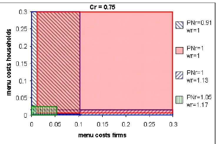
Figure 3: Stable equilibria for Cr = 0:75

= 0:4, = 0:25, = 1=3, = 6, = 2, = 2=3, Cr = 0:75, PT r = 2.

Compared with Figure 1, the most important di¤erence is that the area

corresponding to the menu cost values for which there is an equilibrium, at

which all agents adjust, has shrunk. In Figure 1 it took up the entire area

visible on the graph (I didn’t designate the corresponding zone in order not

to overburden the …gure). Here, the corresponding zone (hatched vertically)

is smaller. For example, this equilibrium is no longer obtained if the …rms’

non-tradables do not change their prices much when all agents adjust: they

increase them by only 5%. Thus, when Cr = 0:75 there is not much danger

of an increase of PN r and this increase would be small in any case (but there

is a possibility of a decrease of PN r: the surface (hatched slanting to the left)

corresponding toPN r = 0:91).

If the central bank wants to avoid an increase of PN r, it can do so by

choosing Cr low enough. But how low Cr has to be (that is, how large the

recession needs to be) depends on the credibility of the central bank. If the

central bank is not credible, then it will need to chose aCrlow enough for no

adjustment to be the only possible equilibrium at the given menu cost values

(or at least to exclude equilibria which imply an inordinately large increase

of PN r). If the central bank is credible, then it does not need to reduce Cr

that much (depending on the menu costs, it might not need to reduce Cr at

all) : it is enough that not adjusting belong to the multiple equilibria. This

implies that two identical countries that di¤er only by the credibility of their

central bank can end up with di¤erent Cr after an identical exchange-rate

shock. For example, if the menu cost is 2% for …rms and 4% for households,

then, with the above parameter values, a credible central bank can keep real

credibility would have to decrease real consumption by a large amount. One

could ask what the maximum value ofCrwould be such that the equilibrium

at which all agents adjust is excluded for the above parameter values. Figure

4 (a zoom on the relevant zone) shows, as a function ofCr, the critical menu

costs for …rms and households such that all agents adjust only if menu costs

are smaller than these critical values.

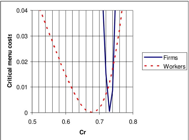
Figure 4: Critical menu costs for the equilibrium at which all

agents adjust

0 0.01 0.02 0.03 0.04

0.5 0.6 0.7 0.8

Cr

Cr

it

ical

m

enu

cost

s

Firms Workers

To exclude the equilibrium at which all agents adjust, it is enough that

one of the menu costs is above the corresponding critical value. When the

menu cost of …rms is 2% and the menu cost of households is 4%, then the

equilibrium at which all agents adjust is excluded at Cr = 0:76. Notice that

the curves are steep: a small change in Cr can have a large impact on the

menu-cost values compatible with all agents adjusting.

7

Conclusion

I have shown that menu costs can explain not only why the price of

non-tradables may remain unchanged after a large devaluation, but also why

it may change by a small amount. I usually obtain multiple equilibria. If

monetary policy is credible, the equilibrium preferred by the central bank

will be selected. If monetary policy is not credible, then the central bank

will have to generate a recession large enough that the equilibrium it wants

to be certain of avoiding is no longer one of the multiple equilibria.

This paper could be extended in several directions. It would be interesting

to extend the model to general equilibrium (for example, foreign demand for

relax simplifying assumptions (for example, the assumption that prices are

fully ‡exible following the …rst period after the shock could be dropped), to

introduce savings and the interest rate (and maybe a monetary policy using

this interest rate as an instrument), to model the cause of the exchange-rate

shock (and its possible links to monetary policy), to integrate substantial

dynamics, and to allow for di¤erent …rms having di¤erent menu costs (idem

for households). One may also want to explain in terms of menu costs faced

by producers of tradables why the price of tradables adjusts whereas the

price of non-tradables adjusts only to a small extent (intuitively, one could

expect that a …rm’s opportunity cost of not adjusting its price is higher in

References

Burstein Ariel, Eichenbaum Martin and Sergio Rebelo (2005a), "Large

Devaluations and the Real Exchange Rate," Journal of Political Economy,

vol. 113(4), pages 742-784, August.

Burstein Ariel, Eichenbaum Martin and Sergio Rebelo (2005b),

"Model-ing Exchange Rate Passthrough After Large Devaluations," Discussion Paper

No. 5250, CEPR, September.

Fishman Arthur and Avi Simhon, (2005) “Can Small Menu Costs Explain

Sticky Prices?”, Economics Letters 87(2), pages 227-230.

Gonzales-Rozada Martín and Pablo Andres Neumeyer (2003), "The

elas-ticity of substitution in demand for non-tradable goods in Latin America

case study: Argentina," mimeo, Universidad T. Di Tella.

Huang Kevin and Zheng Liu (2002), "Staggered price-setting, staggered

wage-setting and business cycle persistence," Journal of Monetary Economics

49, pages 405-433.

of substitution in demand for non-tradable goods in Uruguay," mimeo,

Inter-American Development Bank Research Project.

Midrigan Virgiliu (2006), “Menu Costs, Multi-Product Firms, and

Ag-gregate Fluctuations,” mimeo. January.

Naknoi Kanda (2005), "Real exchange rate ‡uctuations, endogenous