Dynamics of knowledge creation and transfer: The two person case

Munich Personal RePEc Archive

Dynamics of knowledge creation and

transfer: The two person case

Berliant, Marcus and Fujita, Masahisa

Washington University in St. Louis

18 September 2007

Dynamics of Knowledge Creation and

Transfer: The Two Person Case

Marcus Berliant

Masahisa Fujita

September 18, 2007

Abstract

This paper presents a micro-model of knowledge creation and transfer for a couple. Our model incorporates two key aspects of the cooperative process of knowledge creation: (i) heterogeneity of people in their state of knowledge is essential for successful cooperation in the joint creation of new ideas, while (ii) the very process of cooperative knowledge creation a¤ects the heterogeneity of people through the accumulation of knowledge in common. The model features myopic agents in a pure externality model of interaction. In the two person case, we show that the equilibrium process tends to result in the accumulation of too much knowledge in common compared to the most productive state. Equilibrium paths are found analytically, and they are a discontinuous function of initial heterogeneity. JEL Classi…cation Numbers: D83, O31, R11 Keywords: knowledge creation, knowledge transfer, knowledge externalities, endogenous agent heterogeneity

This research owes much to the kind hospitality and stimulating environment of the

Kyoto Institute of Economic Research, where most of our arguments and do-si-do’s occurred.

The …rst author is grateful for funding from the Institute, from Washington University in

St. Louis, and from the American Philosophical Society. The second author is grateful for

Grants Aid for COE Research 09CE2002 and Scienti…c Research Grant S 13851002 from the

Japanese Ministry of Education and Science. We thank Alex Anas, Gilles Duranton, Bob

Hunt, Koji Nishikimi, Diego Puga, Tony Smith, Takatoshi Tabuchi, and seminar participants

at Washington University, New York University, the Spring 2004 Midwest Economic Theory

and International Trade conference, the Federal Reserve Bank of Philadelphia, and the

2004 North American Summer Meetings of the Econometric Society for helpful comments.

Evidently, the authors alone are responsible for any remaining errors and for the views

expressed herein.

Department of Economics, Washington University, Campus Box 1208, 1 Brookings

Drive, St. Louis, MO 63130-4899 Phone: (1-314) 935-8486, Fax: (1-314) 935-4156, e-mail:

[email protected]

Konan University, 8-9-1 Okamoto, Higashinada-ku, Kobe, 658-8501 Japan. Phone and

1

Introduction

In this paper we examine the microdynamics of knowledge creation and trans-fer by using a simple model. With a focus on the two person case, the basic principles of this complex process can be uncovered. Although the two per-son model admittedly has its limitations, particularly in the dynamic choice of partners for knowledge creation and transfer, it has its advantages in ana-lytical tractability because we can solve the equilibrium dynamics explicitly. Elsewhere, in Berliant and Fujita (forthcoming), we provide extensions of the model and results to the context of the general case of any number of potential partners, but to maintain analytical tractability, we do not consider asymmet-ric states or knowledge transfer. In contrast, the latter are the focus of this paper.

Our major research questions are as follows. How do knowledge creation and transfer occur? How do they perpetuate themselves? How do agents change during this process? Are the equilibrium dynamics e¢cient?

As people create and transfer knowledge, they change. Thus, the history of meetings and their content is important. If two people meet for a long time, then their base of knowledge in common increases, and their partnership eventually becomes less productive. Similarly, if two persons have very di¤erent knowledge bases, they have little common ground for communication, so their partnership will not be very productive.

For these reasons, we attempt to model endogenous agent heterogeneity, or horizontal agent di¤erentiation, to look at the permanent e¤ects of knowledge creation and growth. Thus, we are examining how social capital is accumu-lated at a micro level. Our model is analytically tractable, so we do not have to resort to simulations; we …nd each equilibrium path explicitly. The model is also at an intermediate level of aggregation. That is, although it is at a more micro level than large aggregate models such as those found in the endogenous growth literature, we do not work out completely its microfoundations. That is left to future research.

alone. The suitability of a partner dance depends on the stock of knowledge the dancers have in common and their respective stocks of exclusive knowl-edge. The fastest rate of knowledge creation occurs when these factors are in balance.

Our results are summarized as follows. In a two person model where myopic agents can decide whether or not to work with each other, there exist many sink points in the interaction game, depending discontinuously on initial heterogeneity. The most interesting of these features too much homogeneity relative to the most productive state.

For simplicity, we employ a deterministic framework. It seems possible to add stochastic elements to the model, but at the cost of complexity. It should also be possible to employ the law of large numbers to a more basic stochastic framework to obtain equivalent results.

Next we compare our work to the balance of the literature. Section 2 gives the model and notation, Section 3 analyzes equilibrium in the case of two participants or dancers, Section 4 examines welfare in the two person model, whereas Section 5 provides our conclusions and suggestions for future dancing. An appendix provides the proofs of key results.

The basic framework that employs knowledge creation as a black box driving economic growth is usually called the endogenous growth model. Here we make a modest attempt to open that black box. The literature using this black box includes Shell (1966), Romer (1986, 1990), Lucas (1988), Jones and Manuelli (1990), and many papers building on these contributions. There are two key features of our model in relation to the endogenous growth literature. First, our agents are heterogeneous, and that heterogeneity is endogenous to the model. Second, the e¤ectiveness of the externality between agents working together can change over time, and this change is endogenous.

Fujita and Weber (2003) consider a model where heterogeneity between agents is exogenous and discrete. They examine the e¤ects of immigration policy on the productivity and welfare of workers. They note that progress in technology in a country where workers are highly trained is in small steps involving intensive interactions between workers and a relatively homogeneous work force, whereas countries that specialize in production of new knowledge have a relatively heterogeneous work force. This motivates our examination of how endogenous worker heterogeneity a¤ects industrial structure, the speed of innovation, and the pattern of worker interaction.

knowledge is studied in Jovanovic and Rob (1989) in the context of a search model. In contrast, our model examines (endogenous) horizontal heterogene-ity of agents and its e¤ect on knowledge creation, knowledge transfer, and consumption.

2

The Model - Ideas and Knowledge

In this section, we introduce the basic concepts of our model of ideas and knowledge.

An idea is represented by a box. It has a label on it that everyone can read (the label is common knowledge in the game we shall describe). This label describes the contents. Each box contains an idea that is described by its label. Learning the actual contents of the box, as opposed to its label, takes time, so although anyone can read the label on the box, they cannot understand its contents without investing time. This time is used to open the box and to understand fully its contents. An example is a recipe for making “udon noodles as in Takamatsu.” It is labelled as such, but would take time to learn. Another example is reading a paper in a journal. Its label or title can be understood quickly, but learning the contents of the paper requires an investment of time. Production of a new paper, which is like opening a new box, either jointly or individually, also takes time.

Suppose we have an in…nite number of boxes, each containing a di¤erent piece of knowledge, which is what we call an idea. We put them in a row in an arbitrary order.

There are2persons,iandj, in the economy. We assume that each person has a replica of the in…nite row of boxes introduced above, and that each copy of the row has the same order. Our model features continuous time. Fix time t 2 R+ and consider person i. A box is indexed by k = 1;2; :::

Take any box k. If person i knows the idea inside that box, we put a sticker on it that says 1; otherwise, we put a sticker on it that says 0. That is, let xk

i(t) 2 f0;1g be the sticker on box k for person i at time t. The state

of knowledge, or just knowledge, of person i at time t is thus de…ned to be

Ki(t) = (x1i(t); x2i(t); :::) 2 f0;1g

1

. The reason we use an in…nite vector of possible ideas is that we are using an in…nite time horizon, and there are always new ideas that might be discovered, even in the preparation of udon noodles. Given Ki(t) with only …nitely many non-zero components, there is an in…nite

In this paper, we will treat ideas symmetrically. Extensions to idea hier-archies and knowledge structures will be discussed in the conclusions.

GivenKi(t) = (x1i(t); x2i(t); :::),

ni(t) =

1

X

k=1

xk_i(t) (1)

represents the number of ideas known by person i at time t. Next, we will de…ne the number of ideas that two persons, i and j, both know. De…ne

Kj(t) = (x1j(t); x2j(t); :::)and

ncij(t) =

1

X

k=1

xki(t) xkj(t) (2)

Sonc

ij(t) represents the number of ideas known by both persons iand j at

time t. Notice that i and j are symmetric in this de…nition, so nc

ij(t) =ncji(t).

De…ne

nd_ij(t) =ni(t) ncij(t) (3)

to be the number of ideas known by person i but not known by person j at time t.

Knowledge is a set of ideas that are possessed by a person at a particular time. However, knowledge is not a static concept. New knowledge can be produced either individually or jointly, and ideas can be shared with others. But all of this activity takes time.

Next we describe the components of the rest of the model. At each time, each of the two agents faces a decision about whether or not to meet with the other. If both want to meet at a particular time, a meeting will occur. If either does not want to meet, then they do not meet. If the agents do not meet at a given time, then they produce separately and also create new knowledge separately. If the two persons do decide to meet at a given time, then they share older knowledge together and create new knowledge together.

subperiod to produce consumption good on their own, whether or not they are meeting. We shall assume below that although there are no increasing returns to scale in production, the productivity of a person’s labor depends on their stock of knowledge. Activity in the second subperiod depends on whether or not there is a meeting. If there is no meeting, then each person spends the second subperiod creating new knowledge on their own. Evidently, the new knowledge created during this subperiod di¤ers between the two persons, because they are not communicating. They open di¤erent boxes. Since there is an in…nity of di¤erent boxes, the probability that the two agents will open the same box (even at di¤erent points in time), either working by themselves or in distinct meetings, is assumed to be zero. If there is a meeting, then the second subperiod is divided into two parts. In the …rst part, the two persons who are meeting spend their time (and labor) sharing old knowledge, boxes they have opened in previous time periods that the other person has not opened. In the second part, they create new knowledge together, so they open boxes together. We wish to emphasize that the division of a time period into subperiods is purely an expositional device. Rigorously, whether or not a meeting occurs determines how much attention is devoted to the various activities at a given time.

What do the agents know when they face the decision about whether or not to meet at time t? Each person knows both Ki(t) and Kj(t). In other words,

each person is aware of their own knowledge and is also aware of the other’s knowledge. Thus, they also knowni(t),nj(t),ncij(t) = ncji(t),ndij(t), andndji(t)

when they decide whether or not to meet at time t. The notation for whether or not a meeting actually occurs at time t is: ij(t) ji(t) = 1 if a meeting

occurs and ij(t) ji(t) = 0 if no meeting occurs at time t. Meetings only

occur if both persons agree that a meeting should take place.

Next, we must specify the dynamics of the knowledge system and the ob-jectives of the people in the model in order to determine whether or not they decide to meet at a particular time. In order to accomplish this, it is easi-est to abstract away from the notation for speci…c boxes, Ki(t), and to focus

on the dynamics of the quantity statistics related to knowledge, ni(t), nj(t),

nc

ij(t) =ncji(t),ndij(t), andndji(t). Since we are treating ideas symmetrically, in

a sense these quantities are su¢cient statistics for our analysis.

The simplest piece of the model to specify is what happens if there is no meeting and the two people thus work in isolation. Let ai(t) be the rate of

of new ideas created by j, both at time t. Let bij(t) and bji(t) be the rate of

transfer of ideas from i to j and from j to i, respectively, at time t.1 _Then

we assume that the creation of new knowledge during isolation ( ij(t) = 0) is

governed by the following equations:

ai(t) = ni(t) and aj(t) = nj(t) when ij(t) = 0. (4)

bij(t) = 0 and bji(t) = 0 when ij(t) = 0.

So we assume that if there is no meeting at timet, individual knowledge grows at a rate proportional to the knowledge already acquired by an individual. Meanwhile, knowledge held commonly by the two persons does not grow. In particular, ideas are not shared.

If a meeting does occur at timet( ij(t) = 1), then both knowledge exchange

between the two persons and joint knowledge creation occur. When a meeting takes place, joint knowledge creation is governed by the following dynamics:2

aij(t) = [ncij(t) ndij(t) ndji(t)]

1

3 (5)

So when the two people meet, joint knowledge creation occurs at a rate propor-tional to the normalized product of their knowledge in common, the exclusive knowledge of i, and the exclusive knowledge of j. The rate of creation of new knowledge is highest when the proportions of ideas in common, ideas exclusive to person i, and ideas exclusive to person j are split evenly. Ideas in common are necessary for communication, whereas ideas exclusive to one person or the other imply more heterogeneity or originality in the collaboration. If one per-son in the collaboration does not have exclusive ideas, there is no reaper-son for the other person to meet and collaborate. The multiplicative nature of the function in equation (5) drives the relationship between knowledge creation and the relative proportions of ideas in common and ideas exclusive to one or the other agent.

1_{In principle, all of these time-dependent quantities are positive integers. However, for}

simplicity we take them to be continuous (inR+) throughout the paper. One interpretation

is that the creation or sharing of an idea occurs at a stochastic time, and the real numbers are taken to be the probability of a jump in a Poisson process. The use of an integer instead of a real number seems to add little but complication to the analysis.

2_{We may generalize equation (5) as follows:}

aij(t) = max

n

( ")ni(t);( ")nj(t); ncij(t) n d ij(t) n

d ji(t)

1 3o

Under these circumstances, no knowledge creation in isolation occurs. Dur-ing meetDur-ings at time t, knowledge transfer occurs in addition to the creation of new knowledge. Knowledge transfer is governed by the following dynamics:

bij(t) = [ndij(t) ncij(t)]

1

2 (6)

bji(t) = [ndji(t) ncij(t)]

1 2

So when a meeting occurs, knowledge transfer from i to j happens at a rate proportional to the normalized product of the number of ideas that person i

has but that person j does not have, and the ideas common to both persons. The explanation is that communication is necessary for knowledge transfer, so the two persons must have some ideas in common (nc

ij(t)). But in addition,

person i must have some ideas that are not already possessed by person j

(nd

ij(t)). The same intuition applies to knowledge transfer in the opposite

direction from j to i, represented by the second equation in (6). The change in the number of ideas that both persons have in common (n_c

ij(t)) is the sum

of knowledge transfers in both directions and the new ideas jointly created. From personi’s perspective, the number of ideas that ihas butj doesn’t have (nd

ij(t)) decreases with knowledge transfers from i to j. Finally, the change

in the number of ideas possessed by person i is the sum of the ideas that are jointly created and the number of ideas transferred fromj toi. The analogous statements hold for the variables associated with j.

Let us focus on agent i (the equations for agent j are analogous). With a meeting, we have the following dynamics incorporating both knowledge cre-ation and transfer:

_

ni(t) = aij(t) +bji(t)

_

nc_ij(t) = aij(t) +bij(t) +bji(t)

_

nd_ij(t) = bij(t)

Given this structure, we can de…ne the rates of idea innovation and knowl-edge transfer at time t, depending on whether or not a meeting occurs.

_

ni(t) = [1 ij(t)] ni(t) +

ij(t) ( [ncij(t) ndij(t) ndji(t)]

1

3 + [nd

ji(t) ncij(t)]

1 2)

_

nc_ij(t) = ij(t) ( [ncij(t) ndij(t) ndji(t)]

1

3 + [nd

ji(t) ncij(t)]

1 2

+ [ndij(t) ncji(t)]

1 2)

_

nd_ij(t) = [1 ij(t)] ni(t) ij(t) [ndij(t) ncji(t)]

Whether a meeting occurs or not, there is production in each period for both persons. Felicity or instantaneous utility in that time period is de…ned to

be the quantity of output.3 _{De…ne y}

i(t) to be production output (or felicity)

for person i at timet, and de…neyj(t)to be production output (or felicity) of

person j at timet. Normalizing the coe¢cient of production to be 1, we take

yi(t) = ni(t) (7)

so

_

yi(t) = _ni(t)

By de…nition,

_ yi(t)

yi(t)

= n_i(t) ni(t)

(8)

which represents the rate of growth of income.

Finally, we must de…ne the rule used by each person to decide whether they want a meeting at time t or not. Formally,

ij(t) = 1 () (9)

[nc_ij(t) nd_ij(t) nd_ji(t)]13 + [nd

ji(t) ncij(t)]

1

2 > n

i(t) and

[nc_ji(t) nd_ji(t) nd_ij(t)]13 + [nd

ij(t) ncji(t)]

1

2 > n

j(t)

To keep the model tractable in this …rst analysis, we assume a myopic rule. So a person would like a meeting if and only if the increase in their rate of output with a meeting is higher than the increase in their rate of output without a meeting.4 _{Note that we use theincrease in the rate of output rather than the}

rate of output since in a continuous time model, the rate of output at time t

is una¤ected by the decision about whether to meet made at time t.

This completes the statement of the model. Dropping the time dependence of variables to analyze dynamics, we obtain the following equations of motion.

_

yi = _ni = [1 ij] ni+ (10) ij ( [ncij ndij ndji]

1

3 + [nd

ji ncij]

1 2)

_

nc_ij = ij ( [ncij ndij ndji]

1

3 + [nd

ji ncij]

1

2 + [nd

ij ncji]

1 2)

_

nd_ij = [1 ij] ni ij [ndij ncji]

1 2

This system, with analogous equations for agentj, represents a partner dance.

3_{Given that the focus of this paper is on knowledge creation and transfer rather than}

production, we use the simplest possible form for the production function.

3

Equilibrium Dynamics

In order to analyze our system, we …rst divide all of our equations by the total number of ideas possessed byi and j:

nij =nd_ij +nd_ji+nc_ij (11)

and de…ne new variables

mc_ij mc_ji = n

c ij

nij =

nc ji

nij

mdij =

nd ij

nij, m d ji =

nd ji

nij

From (11), we obtain

1 =mdij+mdji+mcij (12)

After some detailed calculations (see Appendix a for all of the steps), we obtain m_d

ij and m_ dji as functions of mdij and mdji only, as follows.

_

md_ij = [1 ij] f(1 mijd)(1 mdij mdji)g (13) ij f [mdij (1 mdij mdji)]

1 2 +md

ij [(1 mdij mdji) mdij mdji]

1 3g

_

md_ji = [1 ij] f(1 mjid)(1 mdij mdji)g ij f [mdji (1 mdij mdji)]

1 2 +md

ji [(1 mdij mdji) mdji mdij]

1 3g

To study this more, we must study (9) further. Deleting time indices and dividing bynij_,

ij = 1 ()

[mc_ij md_ij md_ji]13 + [md

ji mcij]

1

2 > (1 md

ji)

and [mc_ij md_ji md_ij]13 + [md

ij mcij]

1

2 > (1 md

ij)

Substituting further,

ij = 1 ()

[(1 mdji mdij) mdij mdji]

1

3 + [md

ji (1 mdji mdij)]

1

2 > (1 md

ji)

and [(1 md_ji md_ij) md_ji md_ij]13 + [md

ij (1 mdji mdij)]

1

2 > (1 md

ij)

De…ne

Fi(mdij; mdji) = [(1 mjid mdij) mdij mdji]

1

3 + (14)

[md

ji (1 mdji mdij)]

1

2 (1 md

ji)

Fj(mdij; mdji) = [(1 mjid mdij) mdji mdij]

1

3 +

[md_ij (1 md_ji md_ij)]12 (1 md

ij)

and

Mi =f(mdij; mjid)2R2+ jmdij +mdji 1,Fi(mijd; mdji)>0g (15)

Mj =f(mdij; mjid)2R2+ jmdij +mdji 1,Fj(mijd; mdji)>0g (16)

whereas

M =Mi\Mj

The functionFi(mdij; mdji)represents the net bene…t foriof meeting instead

of isolation. Likewise for Fj(mdij; mdji). The set Mi represents those pairs

(md

ij; mdji) such that i wants to meet with j, since for these pairs, the rate of

growth of i’s utility or income with a meeting is higher than the rate of growth of i’s utility or income without a meeting. The set Mj represents those pairs

(md

ij; mdji) such that j wants to meet with i. Of course, the set M represents

those pairs (md

ij; mdji) such that both persons want to meet with each other.

Thus, meetings will occur at time t for pairs inM.

We represent our model in our Figures as a function ofmdij and mdji; since

mdij +mdji +mcij = 1, we know that 1 mcij = mdij +mdji 1, where this

inequality is represented by half of the unit square (a triangle) in R2. We put

mdij on the horizontal axis and mdji on the vertical axis, omitting mc.

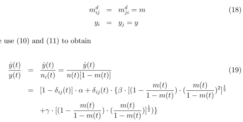
Figure 1, panels (a) and (b) illustrate the sets Mi and Mj, respectively,

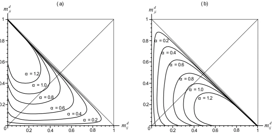
for = = 1 and for various values of . Of course, panels (a) and (b) are mirror images of each other across the 45 line. Figure 2 illustrates M, the set of pairs where both persons want to meet, and its complement, where no meetings occur, for the same parameter values. When(md

ij; mdji)is close to the

boundary of the triangle, meetings do not occur. The reason is that the two persons have too little in common to interact e¤ectively (near the downward sloping diagonal) or someone has too little exclusive knowledge (near the axes) to interact e¤ectively. Meetings only take place in the interior where the three components of knowledge are relatively balanced.

In fact we can describe the properties of the setM in general. The set M

has the shape depicted in Figure 2; see Appendix b for proof. In particular, M

is roughly the shape of an apple core aligned on the 45 line. As increases, the productivity of creating ideas alone increases, so people are less likely to want to meet to create, implying that each Mi and Mj shrinks as increases,

as doesM. If is a little more than1, M disappears. To be precise, letM( )

be the set M under the parameter value . Then, whenever 1 < 2, the set

M( 2) is entirely contained in M( 1). Thus, as shown in Figure 2, there is

a unique point B contained in every M( ), provided M( ) is nonempty. We call B thebliss point, for the pointB in Figure 2 is the point where the rate of increase in income or utility is maximized for each person, as we will explain in the next section (see also Lemma A6 in Appendix c).

Next we discuss the dynamics of the system. Consider …rst the case where there is no meeting, so ij = 0 is …xed exogenously. Then from equations (13),

the dynamics are given by the following equations:

_

md_ij = (1 md_ij)(1 md_ij md_ji) _

md

ji = (1 mdji)(1 mdij mdji)

FIGURE 3 GOES HERE

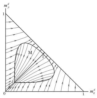
Figure 3, panel (a) illustrates the gradient …eld assuming that ij = 0.

Several facts follow quickly from these derivations. First, if there is no meeting ( ij = 0), then bothm_dij and m_dji are non-negative, and positive on the interior

of the triangle. So if there is no meeting, the vector …eld points to the northeast. Furthermore, in the lower half of the triangle wheremd

ij mdji (the other part

is symmetric), we have

_ md

ji

_ md

ij

= 1 m

d ji

1 md ij

1

where the inequality is strict o¤ of the diagonal. Thus, when ij = 0, the

vector …eld points northeast but toward the diagonal. Under the assumption of no meeting, the system tends to sink points along the diagonal line where

md

ij +mdji = 1, illustrated in Figure 3, panel (a) by a line between (0;1) and

(1;0).

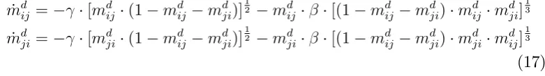
Figure 3, panel (b) illustrates the gradient …eld assuming that ij = 1.

_

md_ij = [md_ij (1 md_ij md_ji)]12 md

ij [(1 mdij mdji) mdij mdji]

1 3

_

md_ji = [md_ji (1 md_ij md_ji)]12 md

ji [(1 mdij mdji) mdji mdij]

1 3

(17)

Both of these expressions are negative on the interior of the triangle and the vector …eld points southwest. Consider, for convenience, the lower half of the triangle where md

ij mdji; the other part is symmetric. Then

_ md

ji

_ md

ij

= [m

d

ji (1 mdij mdji)]

1 2 +md

ji [(1 mdij mdji) mdji mdij]

1 3

[md

ij (1 mdij mdji)]

1 2 +md

ij [(1 mdij mdji) mdij mdji]

1 3

1

where the inequality is strict o¤ of the diagonal. Thus, the vector …eld points southwest but toward the diagonal, as illustrated in Figure 3, panel (b). The only sink is at (0;0), so the system eventually moves there under the assump-tion of a meeting.

Next, we combine the case where there is no meeting ( ij = 0) with the

case where there is a meeting ( ij = 1), and let the agents choose whether or

not to meet. This is illustrated in Figure 4.

FIGURE 4 GOES HERE

The model follows the dynamics for meetings ( ij = 1) on M and the

dynamics for no meetings ( ij = 0) on the complement ofM.

In general, there is a continuum of stable points of the system, correspond-ing to the points wheremd

ij +mdji = 1. For these points, eventually the myopic

return to no meeting dominates the returns to meetings, since eventually the two persons have almost nothing in common. These stable points, however, are not very interesting.

or not meeting at timet, the function ij(t)cannot change its value until time

t+ t. Finally, when at least one person initially happens to be on the bound-ary of M (that is, at least one person is indi¤erent between meeting and not meeting), then they cannot meet for at least t units of time. Under this set of rules, we can be more speci…c about the dynamic process near the boundary of M.

In terms of dynamics, if the system does not evolve toward the uninteresting stable points where there are no meetings (and the two people have nothing in common), eventually the system reaches the southwest boundary of the setM. From there, the assumption that ij is constant over time intervals of at least

length tat the boundary ofM will drive the system in a zigzag process toward the place furthest to the southwest and on the diagonal that is a member of

M. In other words, this is the point J = (mJ_{; m}J_{)2 M with lowest norm. It}

is the remaining stable point of our model. Small movements around J will continue due to our assumption about the dynamics at the boundary of M, namely that meetings or isolation are sticky. As t!0, the process converges to the pointJ. The pointJ features symmetry between the two agents with a large degree of homogeneity relative to the remainder of the points in M and the other points in the triangle generally.

So given various initial compositions of knowledge(md

ij; mdji), where will the

system end up? If the initial composition of knowledge is relatively unbalanced, in other words near the boundary of the triangle, the sink will be a point on the diagonal where md

ij +mdji = 1. If the initial composition of knowledge is

relatively balanced, then the sink will be the point J.

Using the facts about the shape of M, the point J exists and is unique as long as M 6=;.

At the point J = (mJ_{; m}J_{), m}J 2

5, for reasons explained in the next

section.

Without loss of generality, we can allow ij to take values in [0;1] rather

than f0;1g. The interpretation of a fractional ij is that at each instant of

time, a person divides their time between a meeting ij proportion of that

instant and isolation (1 ij) proportion of that instant. All of our results

concerning the model when ij is restricted to f0;1g carry over to the case

where ij 2 [0;1]. The reason is that except on the boundary of M, persons

strictly prefer ij 2 f0;1g to fractional values of ij, as each person’s objective

function is linear in ij. On the boundary ofM, our rule concerning dynamics

the previous iteration of the process for at least time t >0. So if the process pierces the boundary from inside M, it must retain ij = 1 for an additional

time of at least t. If it pierces the boundary from outsideM, it must retain

ij = 0 for an additional time of at least t. It may seem trivial to allow

fractional ij when discussing equilibrium behavior, but allowing fractional ij

is crucial to the next section, where we consider e¢ciency.

4

E¢ciency

To construct an analog of Pareto e¢ciency in this model, we use a social planner who can choose whether or not people should meet in each time period. As noted above, we shall allow the social planner to choose values of ij in[0;1],

so that persons can be required to meet for a percentage of the total time in a period, and not meet for the remainder of the period. To avoid dependence of our notion of e¢ciency on a discount rate, we employ the following alternative concepts. The …rst is stronger than the second. A path of ij is a piecewise

continuous function of time (on [0;1)) taking values in [0;1]. For each path of ij, there corresponds a unique time path of mdij determined by equation

(13), respecting the initial condition, and thus a unique time path of income

yi(t; ij). We say that a path

0

ij (strictly) dominates a path ij if

yi(t;

0

ij) yi(t; ij)and yj(t;

0

ij) yj(t; ij) for all t 0

with strict inequality for at least one over a positive interval of time. As this concept is quite strong, and thus di¢cult to use as an e¢ciency criterion, it will sometimes be necessary to employ a weaker concept, which we discuss next. We say that a path ij is overtaken by a path

0

ij if there exists at

0

such that

yi(t;

0

ij) yi(t; ij) and yj(t;

0

ij) yj(t; ij) for all t > t

0

with strict inequality for at least one over a positive interval of time.

Two types of sink points were analyzed in the last section. First consider equilibrium paths that havemJ _{as the sink point; they reachm}J _{in …nite time}

and stay there. Using Figure 5, we will construct an alternative path 0_ij that dominates the equilibrium path ij.

In constructing this path, we will make use of income changes along the upward sloping diagonal in Figure 4. Setting

md_ij = md_ji=m (18)

yi = yj =y

we use (10) and (11) to obtain

_ y(t) y(t) =

_ y(t) ni(t)

= y(t)_

n(t)[1 m(t)] (19)

= [1 ij(t)] + ij(t) f [(1

m(t) 1 m(t)) (

m(t) 1 m(t))

2_]1 3

+ [(1 m(t) 1 m(t)) (

m(t) 1 m(t))]

1 2)g

To simplify notation, we de…ne the growth rate when the two persons meet,

ij = 1, as

g(m) = [(1 m 1 m) (

m 1 m)

2_]1

3 (20)

+ [(1 m 1 m) (

m 1 m)]

1 2)

Thus

_ y(t)

y(t) = [1 ij] + ij g(m) (21)

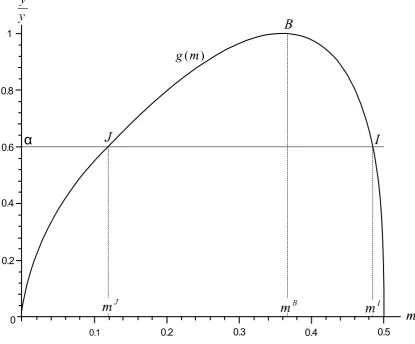
Figure 5 illustrates the graph of the function g(m) as a bold line for = = 1. We can show5 _{that g(m) is strictly quasi-concave on [0;}1

2], achieving

its maximal value at mB _{2 [}1 3;

2

5]. We can also show (see Lemma A6 of the

appendix) that m=mB _{corresponds to the bliss pointB in Figure 2. In other}

words, whenever M 6= ;, B = (mB_{; m}B_{) 2 M, so the point J = (m}J_{; m}J₎

de…ned in Figure 4 and in the previous section has the property thatmJ _2=5,

as it is de…ned to be the point inM on the diagonal and closest to the origin. We de…ne the point I = (mI_{; m}I_{) in Figure 4 to be the point in M on the}

diagonal and farthest from the origin. Lett0

be the time at which the equilibrium path reaches(mJ_{; m}J_{). Let the}

planner set 0

ij(t) = ij(t) for t t0, taking the same path as the equilibrium

path until t0

. From this time on, the planner uses only symmetric points, namely those on the upward sloping diagonal in Figure 4; these points comprise the horizontal axis in Figure 5. At time t0

, the planner takes 0

(mI_{; m}I_{) is attained, prohibiting meetings so that the dancers can pro…t from}

ideas created in isolation. Then the planner sets 0_ij(t) = 1 until (mJ_{; m}J₎

is attained, requiring meetings and the development of more knowledge in common. The last two phases are repeated as necessary.

From Figure 5, the income paths yi(t;

0

ij) and yj(t;

0

ij) generated by the

path 0_ij clearly dominate the income pathsyi(t; ij)and yj(t; ij)generated by

the equilibrium path ij. Thus, the equilibrium path is far from the most

productive path.

Next consider equilibrium paths ij(t)that end in sink points on the

down-ward sloping diagonal in Figure 4. Our dominance criterion cannot be used in this situation, since for potentially dominating plans, the planner will need to force the couple to meet outside of regionM in Figure 4 in early time periods. During this time interval, the dancers could do better by not meeting, and thus a comparison of the income derived from the paths would rely on the discount rate, something we are trying to avoid. So we will use our weaker criterion here, that of overtaking.

Given an equilibrium path ij(t)with sink point on the diagonal, the

plan-ner can construct an overtaking path 0

ij(t) as follows. The …rst phase is to

construct a path 0

ij(t)that reaches a point in region M in …nite time. Such a

path can readily be constructed using Figures 3 and 4.6 _{After reaching region}

M, the second and third phases are the same as described above for the con-struction of a path that dominates one ending with mJ_{. Since the paths with}

sinks on the downward sloping diagonal have income growth at every time, whereas the new path 0

ij(t) features income growth that exceeds whenever

the couple is meeting, 0

ij(t)overtakes ij(t).

The most productive state mB _{is characterized by less homogeneity than}

the stable point mJ_{. Of course, attaining m}B _{requires the social planner to}

force the two persons not to meet some of the time. Otherwise, the system evolves toward more homogeneity.

6_{Such a path can be constructed as follows. In Figure 2 or Figure 4, take the union of}

all closed, one dimensional intervals parallel to the 45 line with one endpoint on an axis and the other endpoint a member of M. Call this setM0_{. From time0, take = 1. Using}

Figure 3(b), the path hitsM0 _{in …nite time. From this time on, take = 0. Using Figure}

5

Conjectures and Conclusions

We have considered a model of knowledge creation and exchange that is based on individual behavior, allowing myopic agents to decide whether joint or individual production is best for them at any given time. This is a pure externality model of knowledge creation, with no markets.

In the present context of two people, there are a continuum of sink points (equilibria) for the knowledge accumulation process. Every state where the two agents have a negligible proportion of ideas in common is attainable as an equilibrium for some initial condition. There is one additional and more interesting sink, involving a large degree of homogeneity as well as symmetry of the two agents, and this is attainable from a non-negligible set of initial conditions. Relative to the e¢cient state, the …rst set of sink points has agents that are too heterogeneous, while the second sink point has agents that are too homogeneous.7

Of course, the major limitation of this work is the use of only two people. In other work, we employ more agents, but at a cost, namely the absence of knowledge transfer while limiting ourselves to symmetric states.

Here we discuss the many alternate directions for future work and exten-sions of the framework. Chief among these are the introduction of foresight on the part of agents, the introduction of stochastic elements into the model, and the introduction of side payments. Though the two person model is limited, extensions of this basic framework are much easier than when there are more persons. It is apparent from the analysis in section 3 that limited foresight, in the form of short sightedness instead of perfect myopia, will not be enough to overturn our results. In order to completely overturn the results of section 2, the agents must have long range foresight. In this case, they can construct more e¢cient paths as in section 3. Moreover, long range foresight in com-bination with side payments could produce tutelage when the initial state is asymmetric. When the person with more knowledge is willing to accept pay-ment for teaching, the equilibrium paths can look very di¤erent from what we have proposed.

In the international context, where each country is often represented by one agent, our model might be applicable. Two countries or two regions would be assigned representative agents. In that context, knowledge creation and transfer, especially as related to developed and developing countries, would be

of interest. Analogs of the transfer paradox would be quite fascinating.8

References

[1] Berliant, M., Fujita, M., forthcoming. Knowledge creation as a square dance on the Hilbert cube. Mimeo. To appear in the International Eco-nomic Review.

[2] Fujita, M., Weber, S., 2003. Strategic immigration policies and welfare in heterogeneous countries. Discussion Paper No. 569, Kyoto Institute of Economic Research, Kyoto University.

[3] Jones, L., Manuelli, R., 1990. A convex model of equilibrium growth: The-ory and policy implications. Journal of Political Economy 98, 1008–1038.

[4] Jovanovic, B. and R. Rob, 1989. The growth and di¤usion of knowledge. The Review of Economic Studies 56, 569-582.

[5] Lucas, R. E., Jr., 1988. On the mechanics of economic development. Journal of Monetary Economics 22, 2–42.

[6] Romer, P., 1986. Increasing returns and long-run growth. Journal of Polit-ical Economy 94, 1002–1037.

[7] Romer, P., 1990. Endogenous technological change. Journal of Political Economy 98, S71–S102.

[8] Shell, K., 1966. Toward a theory of inventive activity and capital accumu-lation. American Economic Review 61, 62–68.

8_{We refer to our companion paper, Berliant and Fujita (forthcoming), for further}

1

0.8

0.6

0.4

0.2

0 _0.2

0.4 0.6 0.8 1

α= 0.2 α= 0.4 α= 0.6 α= 0.8 α= 1.0 α= 1.2

1

0.8

0.6

0.4

0.2

0 _0.2

0.4 0.6 0.8 1

α= 0.2

α= 0.4

α= 0.6

α= 0.8

α= 1.0 α= 1.2

( a) ( b)

Figure 1: The setsMi and Mj under various values of .

1

0.8

0.6

0.4

0.2

0 _0.2

0.4 0.6 0.8 1

α = 0.2 α = 0.4 α = 0.6

α = 0.8 α = 1.0

0 1 1

0 1

1

(a)_δ = 0 (b)_δ = 1

Figure 3: Dynamics under a …xed value of .

1 1

J

M

0

I

1

0.8

0.6

0.4

0.2

0

0.2 0.3 0.4 0.5

0.1

α

Figure 5: E¢ciency and the bliss point

6

Appendix

6.1

Appendix a

Theorem A1: Knowledge dynamics evolve according to the system:

_

md_ij = [1 ij] f(1 mijd)(1 mdij mdji)g ij f [mdij (1 mdij mdji)]

1 2 +md

ij [(1 mdij mdji) mdij mdji]

1 3g

_

md_ji = [1 ji] f(1 mjid)(1 mdij mdji)g ji f [mdji (1 mdij mdji)]

1 2 +md

ji [(1 mdij mdji) mdji mdij]

1 3g

Proof of Theorem A1: Recalling (3),

and dividing by nij _yields

_ yi

nij =

_ ni

nij = [1 ij] (1 m d ji) + ij ( [mc mdij mdji]

1

3 + [md

ji mc]

1 2)

_ nc

ij

nij = ij ( [m c _md

ij mdji]

1

3 + [md

ji mc]

1 2

+ [md_ij mc]12)

_ nd

ij

nij = [1 ij] (1 m d

ji) ij [mdij mc]

1 2

Substituting (12) formc_,

_ yi

nij =

_ ni

nij = [1 ij] (1 m d ji) + ij ( [(1 mdij mjid) mdij mdji]

1

3 + [md

ji (1 mdij mdji)]

1 2)

_ nc

ij

nij = ij ( [(1 m d

ij mdji) mdij mdji]

1

3 + [md

ji (1 mdij mdji)]

1 2

+ [md_ij (1 md_ij md_ji)]12)

_ nd

ij

nij = [1 ij] (1 m d

ji) ij [mdij (1 mdij mdji)]

Now

_

md_ij = d(n

d ij=nij)

dt = n_

d ij

nij

nd ij n_ij

(nij₎2

= n_

d ij

nij

ndij

nij

_ nij

nij

= [1 ij] (1 mdji) ij [mdij (1 mdij mdji)]

1

2 md

ij ( _ nd ij n + _ nd ji n + _ nc ij n ) = [1 ij] (1 mdji) ij [mdij (1 mdij mdji)]

1 2

md_ij f[1 ij] (1 mdji) ij [mdij (1 mdij mdji)]

1 2 + [1

ij] (1 mdij) ij [mdji (1 mdij mdji)]

1

2 +

ij ( [(1 mdij mjid) mdij mdji]

1 3

+ [md_ji (1 md_ij md_ji)]12 + [md

ij (1 mdij mdji)]

1 2)g

= [1 ij] (1 mdji) ij [mdij (1 mdij mdji)]

1 2

md_ij f[1 ij] (1 mdji) + [1 ij] (1 mdij)

+ ij [(1 mdij mjid) mdij mdji]

1 3g

= [1 ij] f1 mdji 2mdij + (mdij)2+mdij mdjig ij f [mdij (1 mdij mdji)]

1 2 +md

ij [(1 mdij mdji) mdij mdji]

1 3g

= [1 ij] f(1 mdij)(1 mjid) mdij+ (mdij)2g ij f [mdij (1 mdij mdji)]

1 2 +md

ij [(1 mdij mdji) mdij mdji]

1 3g

= [1 ij] f(1 mdij)(1 mjid) mdij(1 mdij)g ij f [mdij (1 mdij mdji)]

1 2 +md

ij [(1 mdij mdji) mdij mdji]

1 3g

= [1 ij] f(1 mdij)(1 mdji mdij)g ij f [mdij (1 mdij mdji)]

1 2 +md

ij [(1 mdij mdji) mdij mdji]

1 3g

The fourth line follows from (11), that implies

_ nij

nij =

_ nd

ij

nij +

_ nd

ji

nij +

_ nc

ij

nij (22)

Symmetric calculations hold for m_d ji.

6.2

Appendix b

Theorem A2: Suppose that (md

ij; mdji) 2 M. Then (mdji; mdij) 2 M and

the line segment [(md

ij; mdji);(mdji; mijd)] M. In particular, if M 6=;, then it

intersected with M is a convex set. Finally, every point in M \((0;0);(1;1))

has a neighborhood contained in M.

To prove Theorem A2, we proceed with a …nite sequence of lemmata. First we need some de…nitions to make notation easier.

De…nitions:

f(m; m0

) = [(1 m m0

) m m0

]13

h(m; m0) = [(1 m m0) m0]12

With these de…nitions, the equations de…ningMi (15) andMj (16) become:

f(md_ij; md_ji) +h(md_ij; md_ji) (1 md_ji)>0 (23)

f(md_ji; md_ij) +h(md_ji; md_ij) (1 md_ij)>0 (24)

Lemma A1: (md

ij; mdji) 2 Mi and mdij mdji imply (mdji; mdij) 2 Mi.

(md

ij; mdji)2Mj and mdij mdji imply (mdji; mdij)2Mj.

Proof of Lemma A1: f(md

ij; mdji) =f(mdji; mdij). h(md

ji;mdij)

h(md

ij;mdji) = [

md ij

md ji]

1

2 1,

since md

ij mdji. (mdij; mdji) 2 Mi implies f(mdij; mdji) +h(mdij; mdji) (1

md

ji) > 0. Since h(mdji; mdij) h(mdij; mjid) and mdij mdji, f(mdji; mdij) +

h(md

ji; mdij) (1 mdij)>0. Hence,(mdji; mdij)2Mi. A symmetric argument

works for the second part of the lemma.

Lemma A2: Suppose that md

ij mdji. Then (mdij; mdji)2M if and only if

(md

ij; mdji)2Mi.

Proof of Lemma A2: It is obvious that(md

ij; mdji)2M implies(mdij; mdji)2

Mi. So suppose that (mdij; mdji) 2 Mi. Then by symmetry of the

de…ni-tions of Mi and Mj, (mdji; mdij) 2 Mj. By Lemma A1, (mdji; mdij) 2 Mi.

Applying symmetry of the de…nitions again yields (md

ij; mdji) 2 Mj. Hence

(md

ij; mdji)2Mj \Mi =M.

Lemma A3: Suppose that (md

ij; mdji) 2 M. Then (mdji; mdij) 2 M and

the line segment [(md

ij; mdji);(mdji; mijd)] M. In particular, if M 6=;, then it

contains a point on the diagonal segment [(0;0);(1;1)].

Proof of Lemma A3: First, if (md

ij; mdji) 2 M, then (mdji; mdij) 2 M

by symmetry of the de…nitions of Mi and Mj. Now consider the line

seg-ment [(md

ij; mdji);(mdji; mijd)]. In particular, consider the case mdij mdji and

the line segment between (md

ij; mdji) and the point (m; m) on the diagonal,

[(md

ij; mdji);(m; m)] [(mdij; mdji);(mdji; mdij)](the line segment[(m; m);(mdji; mdij)]

can be covered with a symmetric argument). Since for all(m_bd

b

md

ij mbdji, by Lemma A2 it su¢ces to show that (mbijd;mbdji) 2 Mi. We must

verify the equation stating that (m_bd

ij;mbdji)2Mi, namely

f(m_bd_ij;m_bd_ji) +h(m_bijd;m_bd_ji) (1 m_bd_ji)>0 (25) Now for all (m_bd

ij;mbdji)2 [(mdij; mdji);(m; m)], there exists an x 0with mbdij =

md

ij x mdji+x=mbdji, since the line segment lies below the diagonal. Now

f(md_ij x; md_ji+x) f(md_ij; md_ji)

= [(1 md_ji md_ij) (m_ijd x) (md_ji+x)]13 [(1 md

ji mdij) (mdij) (mdji)]

1 3

= [(1 md_ji md_ij) (md_ij) (md_ji) + (1 md_ji md_ij) x (md_ij md_ji x)]13

[(1 md_ji md_ij) (md_ij) (md_ji)]13

[(1 md_ji md_ij) (md_ij) (md_ji) + (1 md_ji md_ij) x2]13

[(1 md_ji md_ij) (md_ij) (md_ji)]13

0

h(md_ij x; md_ji+x) h(md_ij; md_ji)

= [(md_ji+x) (1 m_jid md_ij)]12 [md

ji (1 mdji mdij)]

1

2 0

Finally,

(1 md_ji x) (1 md_ji)

Hence,

f(m_bdij;mbdji) +h(mbdij;mbdji) (1 mbdji)

= f(md_ij x; md_ji+x) +h(m_ijd x; md_ji+x) (1 md_ji x) f(mdij; mdji) +h(mdij; mdji) (1 mdji)>0

The last line follows because (md

ij; mdji)2M.

Lemma A4: For any constant a 2 ( 1;1) the intersection of the set M

and the line f(md

ij; mdji)2R2+ jmdij +mdji 1, mdji =mdij ag is a convex set.

Proof of Lemma A4: SinceM is symmetric with respect to the diagonal

md

ij =mdji, let us consider a 0. Setting mdji =mdij a in (14), de…ne

k(md_ij) Fi(mdij; mdij a)

= (1 +a 2md_ij)md_ij(md_ij a) 1=3

+ (1 +a 2md_ij)(md_ij a) 1=2 (1 +a md_ij)

Since md

ji = mdij a 0 and 1 mdij +mdji = 2mdij a, the domain of the

function k is

a md_ij 1 +a

By Lemma A2, the intersection of the setM and the linemd

ji =mdij a is the

set of points satisfying

k(md_ij)>0:

We show that function k(md

ij)is strictly concave on (a;1+2a), and thus the set

of points satisfying the inequality is convex. Di¤erentiation of the function k

yields

k0

(md_ij) = A(md_ij) +B(md_ij) +

where

A(md_ij)

3 (1 +a 2m

d

ij)mdij(mdij a)

2=3

6(md_ij)2+ 2md_ij(1 + 3a) a(1 +a)

B(md_ij)

2 (1 +a 2m

d

ij)(mdij a)

1=2

(1 + 3a 4md_ij)

The second derivative of k is

k00(md_ij) = A0(md_ij) +B0(md_ij)

where

A0

(md_ij) = 2 (m

d

ij)2(1 + 3a2) a(1 +a)(1 + 3a)mdij +a2(1 +a)2

9 (1 +a 2md

ij)mdij(mdij a)

5=3

=

2 hmd

ij(1 + 3a2)

a(1+a)(1+3a) 2

i2

+3a2(1+a₄)2(1 a)2

9 (1 +a 2md

ij)mdij(mdij a)

5=3

(1 + 3a2₎

B0(md_ij) = (1 a)

2

4 (1 +a 2md

ij)(mdij a)

3=2

implying that k00

(md

ij) = A

0

(md ij) +B

0

(md

ij) < 0 on (a;1+2a), so k is strictly

concave on (a;1+a

2 ). Thus, fm

d

ij 2 (a;1+2a) j k(m

d

ij) > 0g is convex, and the

proof of the lemma is complete.

Lemma A5: Every point in M \((0;0);(1;1)) has a neighborhood con-tained in M.

Proof of Lemma A5: This follows directly from the de…nition of M; it implies that M is an open set.

6.3

Appendix c

Lemma A6: The function g(m) de…ned by (20) has the following properties: (i) g(m) is strictly quasi-concave on 0;1₂ .

(ii) g(m) achieves its maximal value at mB _2[1 3;

2 5].

(iii) The point (mB_{; m}B_{)corresponds to the bliss point B in Figure 2, which}

is the unique point contained in every M that is nonempty.

Proof of Lemma A6: (i) and (ii): For m2 0;1₂ , let

x(m) m

1 m or m(x) = x 1 +x

and de…ne

G(x) (1 x)x2 1=3+ [(1 x)x]1=2 for x2[0;1] (26)

Then, using de…nition (20)

g(m) = G(x(m))

Hence,

g0

(m) =G0

(x(m)) x0

(m)

Notice that

x0

(m) = 1 + m

(1 m)2 >0

so

g0

(m)_R0exactly as G0

(x(m))_R0. Now

G0(x) = C(x) +D(x)

where

C(x) ₃[(1 x)x2_] 2=3_{(2 3x)x}

D(x) ₂[(1 x)x] 1=2(1 2x)

Taking the derivatives of C and D respectively yields

C0

(x) = 2₉ (1 x) 5=3_x 4=3 _<0

D0

(x) = ₄(1 x) 3=2_x 3=2 _<0

Therefore, considering that

we can conclude that there exists a unique x 2[1=2;2=3] such that

G0

(x)R0 asxQx

meaning that G is strictly single peaked and strictly quasi-concave, achieving its maximum value exactly at x . Hence, the function g(m) also is strictly single peaked and strictly quasi-concave, achieving its maximum value at

mB _{m(x ) =} x

1 +x 2[1=3;2=5]

(iii) To show that the point (mB_{; m}B_{) corresponds to the bliss point B in}

Figure 2, let us recall how the bliss point has been de…ned. Let M( ) be the set M under the parameter value > 0. Then, a point ( md

ij; mdji) 2 R2 is

called a bliss point if it holds that for any >0,

M( )6=;=)( md_ij; md_ji)2M( ) (27)

To show the existence and the uniqueness of such a point, since M( ) is symmetric to the upward sloping diagonal, let us focus on the lower half of

M( ), and de…ne

ML( ) = (md_ij; md_ji)2M( )jmd_ij md_ji

Then, by Lemma A2, ML_{( ) coincides with the lower part of M}

i associated

with :

ML_{( ) = (m}d

ij; mdji)2Mi( )jmdij mdji

=f(md

ij; mdji)2R2 jmijd mdji 0; mdij +mdji 1;

f(md

ij; mdji) +h(mdij; mjid) (1 mdji)>0g

When md

ij +mdji = 1 or mdji = 0, we have f(mdij; mdji) = h(mdij; mdji) = 0,

implying that ML_{( ) does not contain any point (m}d

ij; mdji) such that mdij +

md

ji = 1 ormdji = 0. Thus, we can rewriteML( ) as follows:

ML_{( ) =}n_(md

ij; mdji)2R2 jmdij mdji >0; mdij+mdji <1; f(md

ij;mdji)

1 md

ji +

h(md ij;mdji)

1 md ji >

o

=f(md

ij; mdji)2R2 jmdij mdji >0; mdij+mdji <1; h

1 m

d ij

1 md ji

md ij

1 md ji

md ji

1 md ji

i1=3

+ h 1 m

d ij

1 md ji

md ji

1 md ji

i1=2

> g (28) Given any (md

ij; mdji)2ML( )such that mdij > mdji, de…ne

m m

d

ij +mdji

Then, md

ij > m > mdji, and (m; m)2ML( ) by Lemma A3. Furthermore,

1 m 1 m m 1 m 2 1 m d ij

1 md ji

!

md ij

1 md ji

md ji

1 md ji

= (1 m

d

ij mdji)m2

(1 m)3

(1 md

ij mdji)mdijmdji

(1 md ji)3

> (1 m

d

ij mdji)

(1 md ji)3

(m2 _md ijmdji)

= (1 m

d

ij mdji)

(1 md ji)3

(md

ij mdji)2

4 >0

Likewise,

1 m 1 m

m

1 m 1

md ij

1 md ji

!

md ji

1 md ji

= (1 m

d

ij mdji)m

(1 m)2

(1 md

ij mdji)mdji

(1 md ji)2

> (1 m

d

ij mdji)

(1 md ji)2

(m md_ji)>0

Therefore, using the functiong(m)de…ned by (20), we can conclude that when

md

ij > mdji and m (mdij +mdji)=2,

g(m)>

"

1 m

d ij

1 md ji

!

md ij

1 md ji

md ji

1 md ji

#1=3

+

"

1 m

d ij

1 md ji

!

md ji

1 md ji

#1=2

(29) Moreover, (i) and (ii) of Lemma A6 mean that

g(mb)> g(m) for any m6=mb (30)

Combining (28), (29) and (30), we can conclude that given any(md

ij; mdji)such

that md

ij mdji

(md_ij; md_ji)2ML( ) =)(mB; mB)2ML( ).

That is,

ML( )6=;=)(mB; mB)2ML( ) (31) Hence, the point(mB_{; m}B_{)is a bliss point. Finally, to show that the bliss point}

is unique, take any > 0 such that ML_{( ) 6= ;, and take any (m}d

ij; mdji) 2

ML_{( ) such that (m}d

(29) holds when (md

ij; mdji) is replaced with (mdij; mjid). If mdij = mdji, then

g(mB_{)> g(m}d

ij) by (30). Hence, if we de…ne

" g(mB)

8 < :

"

1 m

d ij

1 md ji

!

md ij

1 md ji

md ji

1 md ji

#1=3

+

"

1 m

d ij

1 md ji

!

md ji

1 md ji

#1=29₌

;

then " is positive. Replacing with g(mB₎ "

2 and (m

d

ij; mdji) with (mdij; mdji)

in (28), we can see that

(md_ij; md_ji)2= ML g(mB) " 2

whereas (mB_{; m}B_{) 2M}L _g(mB₎ "

2 . Thus, the point (m

d

ij; mdji) is not

con-tained in the nonempty setML _g(mB₎ "

2 , implying that the point(m

d

ij; mdji)6=