Generation of an Effective Training Feature Vector using VQ for Classification of Image Database

Generation of an Effective Training Feature Vector using

VQ for Classification of Image Database

H. B. Kekre

Professor, Computer Engineering, Mukesh Patel

School of Technology Management and Engineering, NMIMS University, Vileparle(w)

Mumbai 400056, India

Tanuja K. Sarode

Associate Professor, Computer Engineering, Thadomal Shahani

Engineering College, Bandra(W), Mumbai 400050,

India

Jagruti K. Save

Ph.D. Research Scholar, MPSTME, NMIMS University, Associate Professor, Computer

Engineering, Fr. C. Rodrigues College of Engineering, Bandra(W), Mumbai 400050,

India

ABSTRACT

In supervised classification of image database, feature vectors of images with known classes, are used for training purpose. Feature vectors are extracted in such a way that it will represent maximum information in minimum elements. Accuracy of classification highly depends on the content of training feature vectors and number of training feature vectors. If the number of training images increases then the performance of classification also improves. But it also leads to more storage space and computation time. The main aim of this research is to reduce the number of feature vectors in an effective way so as to reduce memory space required and computation time as well as to increase an accuracy. This paper proposes three major steps for automatic classification of image database. First step is the generation of feature vector of an image using column transform, row mean vector and fusion method. Then vector Quantization (code book size 4,8 and 16) is applied to reduce the number of training feature vectors per class and generate an effective and compact representation of them. Finally nearest neighbor classification algorithm is used as a classifier. The experiments are conducted on augmented Wang database. The results for various transforms, different similarity measures, varying sizes of feature vector, three code book sizes and different number of training images, are analyzed and compared. Results show that the proposed method increases accuracy in most of the cases.

General Terms

Image Classification, Vector quantization, Algorithms, Image Database.

Keywords

Supervised Classification, Row Mean Vector, Similarity Measures, Nearest Neighbor Classifier, Feature Vector.

1.

INTRODUCTION

Automatic Image Classification has become more important with the development of Internet and the growth in the size of image databases. It is a process of assigning images to a number of predefined categories. For large databases, classification or categorization of images is an useful preprocessing step for image retrieval system. A successful classification of images will greatly enhance the performance of content-based image retrieval systems by filtering out images from irrelevant classes during matching (A.Vailaya et al. 1998)[1]. Due to the content heterogeneity that exist among the different images which are downloaded from the internet, their automatic classification has become a great challenge. Classification of images is of two types : Supervised and Unsupervised. In Supervised classification,

the training set (set of images with their classes) is available. In unsupervised classification, no such training set is available. Unsupervised classification is also known as clustering. This paper proposes the technique for supervised classification. Most of the classification systems generate image feature vectors for dimension reduction and as a representation of an image. Feature extraction is an important issue for generic image classification. So lot of research has been done in this area. N.Manshor et al. 2012, proposed the combination of different low level features with local features for improving the performance of object class recognition[2]. H.Nakayama et al. 2009, increased the performance of global features by using local feature correlation[3]. D.Choudhary et al. 2013, has shown that the wavelet features can be used to generate feature vector[4]. The combination of local and global properties can also be considered to generate feature vectors (W.H.Cho et al. 2013)[5]. These extracted features are applied to classifiers such as nearest neighbor classifier(O. Boiman et al. 2008)[6], decision tree classifier and Bayes classifier. Artificial neural network (ANN) and Support vector machine (SVM) are also popular methods for classification (M.W.Ashour et al. 2013)[7]. Li Fei-Fei et al. 2005, proposed a Bayesian hierarchical model to learn and recognize natural scene categories[8]. S.D.M. Raja et al. 2011,has given comparison of ANN and SVM based classifiers[9].

problem, we have suggested to generate an effective representation from those training images. This representation contains few number of training feature vectors. For classification stage, nearest neighbor classifier is implemented. To find the closest feature vector, different similarity measures such as Euclidean distance, Manhattan distance(E.Deza et al 2006)[17] (John P. et al. 1995)[18], Cosine correlation similarity and Bray-Curtis similarity (S.Santini et al. 1999)[19], (H.B.kekre et al. 2012)[20] have been used. The paper is organized as follows : Section 2 explains LBG (Linde-Buzo-Gray,1980)[21] (R.M.Gray, 1984)[22] vector quantization method. Section 3 gives detailed procedure of proposed system. Section 4 shows all the results of implementation followed by conclusions and future scope in section 5 and references in section 6.

2.

LINDE-BUZO-GRAY ALGORITHM

In 1980, Linde et al. proposed a Generalized Lloyd Algorithm (GLA) which is also called Linde-Buzo-Gray (LBG) algorithm. This algorithm is applied on all training feature vectors of each class. Consider the classes are numbered as C1,C2,...,C20.

The LBG algorithm steps are as follows : For Class C1 to C20 do

BEGIN

1. All training feature vectors of the class belong to one cluster.

2. Calculate the centroid of all vectors. This is the first code vector.

3. Addition and subtraction of constant error with the code vector forms two trial code vectors say v1 and v2. Assume these vectors represent two clusters.

4. Find the closeness for each training vector in a cluster with these two trial code vectors. Put the feature vectors in an appropriate cluster. Thus initial single cluster is divided into two clusters.

5. Calculate the centroid for each cluster. These are two code vectors.

6. Repeat the steps 3 to step 5 for each cluster till the desired number of code vectors generated. After every iteration each cluster gets divided into two clusters. 7. Store these code vectors.

END

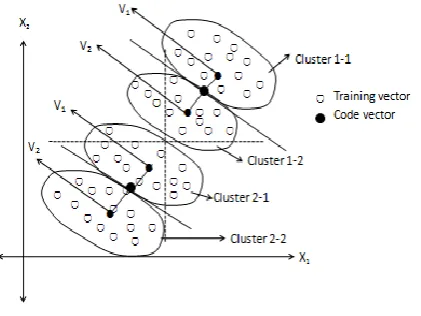
Figure 1(a) & (b) shows the LBG procedure representation for two dimensional training vectors.

Figure 1(a) LBG for two dimensional case after two clusters formation

Figure 1(b) LBG for two dimensional case after four

clusters formation

3.

PROPOSED ALGORITHM

The proposed method can be divided into 3 sections. Section 3.1 explains generation of feature vector for training image. Same method is used to generate the feature vector of each testing image. Section 3.2 gives the procedure to generate 4,8 and 16 representative training feature vectors for each class using LBG vector quantization. Finally section 3.3 gives the method of classification of test image.

3.1

Generation of Feature vector for each

Training Image

Image is resized to 256x256. Apply image transform ( such as DCT, DST, DFT, DHT, DWT and DKT) to the columns of R,G and B plane of an image. Calculate the average of each row of a plane. This will generate the row mean vector for each plane. These row mean vectors are organized one below the other as shown in figure 2 to generate the feature vector. The size of each row mean vector is 256x1. The size of feature vector depends on the number of elements taken from the row mean vectors. If all elements of row mean vectors are taken, then the size of feature vector is 768x1. If only first 25 elements of each row mean vector is considered, then the feature vector of size 75x1 will be generated. Thus different sizes of feature vectors such as 150x1, 300x1, 450x1, 600x1 are also tried and tested their impact on the accuracy.

Figure 2. Generation of feature vector

3.2

Generation of Representative Training

Feature Vectors for Each Class

Figure 3. Code vector generation

3.3

Classification of Test image

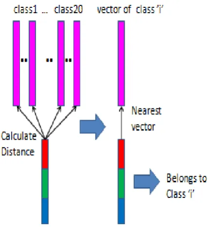
For a test image, feature vector is generated using the procedure in section 3.1. Nearest neighbor algorithm is used for classification. The training feature vector closest to the test feature vector is found out and the test image is assigned to the corresponding class of that training feature vector as shown in figure 4. To find the closeness of feature vectors, different similarity criteria such as Euclidean distance, Manhattan distance, Cosine correlation and Bray-Curtis similarity are used.

Fig.4. Classification of test image

4.

RESULTS AND DISCUSSION

The implementation of the proposed method is done in MATLAB 7.0 using a computer with Intel Core i5, CPU (2.50GHz and 6 GB RAM). The proposed techniques are tested on the Augmented Wang database (J.Z.Wang et al. 2001)[23]. Six classes (Dinosaur, Horse, Rose, Elephant, Mountains and Bus) are directly taken from Wang database. Remaining 14 classes are downloaded from internet. Each class contains 100 images. Total images in database are 2000. Figure 5 shows the sample images of Training database. Figure 6 shows the sample images of testing database.

Figure 5. Sample Images of Training Database

Figure 6. Sample Images of Testing Database

Table 1. %Accuracy of correctly classified images

Feature vector size= 100G+100R+100B (300 x1) Traini ng Images : 700

Transform Similarity Criteria

Number of training vectors/class

1 4 8 16 35

(Average) (LBG-4) (LBG-8) (LBG-16) (All)

DCT

Euclidean 47.23 52.85 55.31 55.54 57.69

Manhattan 52.54 55.46 58.92 60.46 57.23

Cosine

Correlation 51.62 53.15 55.15 54.46 56.46

Bray-Curtis 52.15 56 59.85 60.62 57.46

DST

Euclidean 51 58.77 59.31 59.15 59.54

Manhattan 52.85 61.31 62.15 62.85 60.23

Cosine

Correlation 55.15 59.62 62.08 61.38 61.38

Bray-Curtis 52.62 62.38 63.15 63.62 60.38

DFT

Euclidean 43.77 50.92 53.85 53.23 53.23

Manhattan 49.31 52.23 55.38 56.08 55.23

Cosine

Correlation 48.69 51.46 53.77 52.92 51.54

Bray-Curtis 49.23 51.85 56.23 56.62 55

DHT

Euclidean 43.46 51.31 51.31 52.85 50.54

Manhattan 48.92 54 55.92 55.54 53.38

Cosine

Correlation 47.54 49.38 50.92 50.08 49.46

Bray-Curtis 49 53.62 55.69 56.92 53.15

DWT

Euclidean 45.6 50.31 53.54 54.08 55.6

Manhattan 51.7 53 58 57.85 55.85

Cosine

Correlation 51.31 51.46 53.77 53.62 55.38

Bray-Curtis 50.69 55.08 59.08 59.23 57

DKT

Euclidean 41.31 45.54 49.08 47.69 50.15

Manhattan 38.92 44.92 49.77 50.46 49.46

Cosine

Correlation 45.69 45.15 46.92 45.54 50.31

Bray-Curtis 39.23 45 49.69 49.62 49.15

Note :Yellow color indicates maximum accuracy achieved for each similarity criteria in each transform. Red color indicates overall maximum accuracy achieved for every transform.

Observations : LBG with code book size of 16 gives highest accuracy in all transforms. In Manhattan and Bray-Curtis similarity, this vector quantization method gives quite high improvement in accuracy. Highest accuracy achieved is

Table 2. %Accuracy of correctly classified images

Feature vector size= 100G+100R+100B (300 x1) Training Images : 1100

Transform Similarity Criteria

Number of training vectors/class

1 4 8 16 55

(Average) (LBG 4) (LBG 8) (LBG 16) (All)

DCT

Euclidean 47.78 54.44 58.67 59.56 60.44

Manhattan 54.44 59.67 61.7 65.9 61.89

Cosine Correlation 50.56 53.56 58.1 60.3 58.33

Bray-Curtis 54.44 60.11 60.6 65.6 62

DST

Euclidean 48.89 58.56 62.22 63.89 63

Manhattan 52.56 62.67 64.33 63.67 60.33

Cosine Correlation 54.56 60.44 63 63.89 61.78

Bray-Curtis 51.56 63.44 65.44 64.78 61.67

DFT

Euclidean 43.78 53.33 55.89 54.67 55.33

Manhattan 49.78 54.22 58.7 60 56.78

Cosine Correlation 50.56 52.33 54.4 57.4 53.89

Bray-Curtis 48.89 55 59.2 60.1 56.67

DHT

Euclidean 48.11 52.89 54.56 54.44 53.22

Manhattan 49.67 54 58.89 58 55.78

Cosine Correlation 51.89 50.22 53 52.56 52.56

Bray-Curtis 49.44 54 58.22 56.56 56.22

DWT

Euclidean 47 52.56 56.78 58.56 60.67

Manhattan 52.67 57.2 61.4 62.67 58.22

Cosine Correlation 51 53.4 57.6 57 57.11

Bray-Curtis 52.56 58.3 61.1 63.11 60.67

DKT

Euclidean 41.89 45.78 49.67 49 51.89

Manhattan 38.67 46.33 47.33 51.33 52.89

Cosine Correlation 46.22 45.78 48.22 47.67 52

Bray-Curtis 38.11 45.67 47.11 51.44 51.67

Note :Yellow color indicates maximum accuracy achieved for each similarity criteria in each transform. Red color indicates overall maximum accuracy achieved for every transform

Observations : In all transforms except DKT transform, highest accuracy is achieved with LBG vector quantization. In Manhattan and Bray-Curtis similarity, this vector quantization method gives quite high improvement in accuracy in most

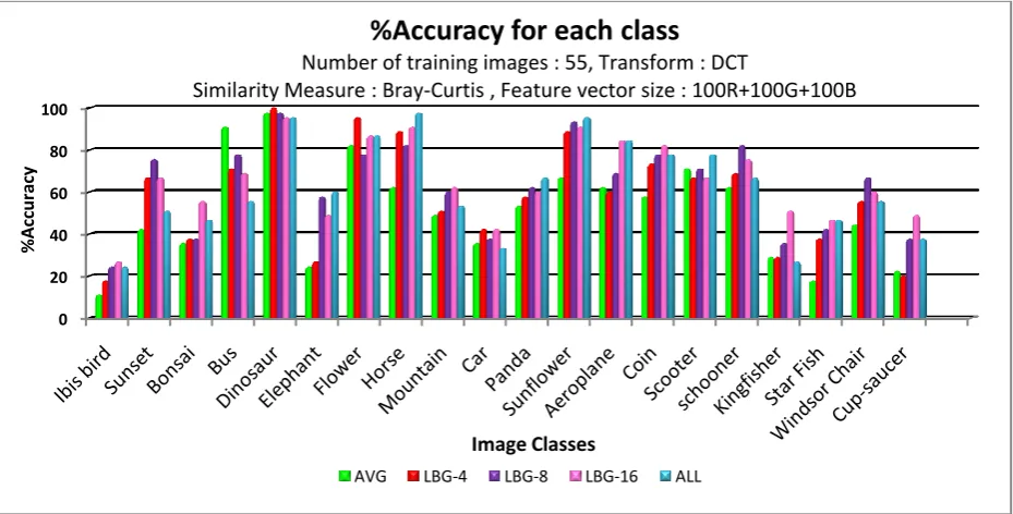
Figure 7. % Accuracy for each individual class Observations: In most of the individual classes such as Ibis

bird, Sunset, Bonsai, Elephant, Mountain, Car, Panda, Coin, Schooner, Kingfisher and Cup-saucer, LBG gives higher

accuracy than 'AVG' and 'ALL' case. In 11 classes, the maximum accuracy achieved is more than 60%

Figure 8. % Accuracy for each individual class Observations: In most of the individual classes such as Ibis

bird, Sunset, Bonsai, Dinosaur, Flower, Mountain, Car, Coin, Schooner, Kingfisher, Windsor Chair and Cup-saucer, LBG

gives higher accuracy than 'AVG' and 'ALL' case. In 14 classes, the maximum accuracy achieved is more than 60%. 0

20 40 60 80 100

%

A

cc

u

rac

y

Image Classes

%Accuracy for each class

Number of training images : 55, Transform : DST

Similarity Measure : Bray-Curtis , Feature vector size : 100R+100G+100B

AVG LBG-4 LBG-8 LBG-16 ALL

0 20 40 60 80 100

%

A

cc

u

rac

y

Image Classes

%Accuracy for each class

Number of training images : 55, Transform : DCT

Similarity Measure : Bray-Curtis , Feature vector size : 100R+100G+100B

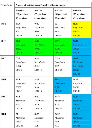
Table 3. Overall highest %accuracy for each transform

Transform Number of training images/ number of testing images

500/1500 (25 per class/

75 per class)

700/1300 (35 per class/

65 per class)

900/1100 (45 per class/

55 per class)

1100/900 (55 per class/

45 per class)

DCT 59.3

Bray-Curtis 300X1 LBG-8 60.62 Bray-Curtis 300X1 LBG-16 62 Bray-Curtis 450X1 LBG-16 65.89 Bray-Curtis 300X1 LBG-16

DST 61.8

Bray-Curtis 450X1 LBG-8 63.62 Bray-Curtis 300X1 LBG-16 63.91 Bray-Curtis 300X1 LBG-16 65.44 Bray-Curtis 300X1 LBG-8

DFT 55.5

Bray-Curtis 300X1 LBG-8 56.62 Bray-Curtis 300X1 LBG-16 58.55 Bray-Curtis 150X1 LBG-16 60.67 Manhattan Bray-Curtis 150X1 LBG-16

DHT 56.4

Bray-Curtis 300X1 LBG-8 58.08 Bray-Curtis 768X1 LBG-16 59.82 Bray-Curtis 768X1 LBG-16 59.22 Bray-Curtis 768X1 LBG-16

DWT 59.4

Manhattan 450X1 LBG-8 59.62 Bray-Curtis 768X1 LBG-16 62.45 Manhattan 300X1 LBG-16 63.22 Manhattan 450X1 LBG-16

DKT 57

Manhattan 768X1 LBG-16 58.69 Euclidean 768X1 ALL 59.27 Manhattan 768X1 ALL 61.78 Manhattan 768X1 LBG-16

Note : Yellow color indicates highest accuracy among all the transforms. Green color indicates highest performance in each column. Blue color indicates highest performance in each row

Observations: For DCT, DST, DFT, DHT and DWT, proposed technique has given the highest accuracy for all cases.

5.

CONCLUSIONS AND FUTURE

SCOPE

The paper presents an approach to generate compact and effective training set from the given training set of feature vectors. After doing a lot of experimentation, we have observed that classification with all training vectors gives far better results than single average training feature vector for each class. This fact has given an idea to make groups of training vectors of same class and select one representation

900 (45 images/class) and 1100 (55 images/class) training feature vectors. Thus the technique significantly reduces the storage space and computation time. It also increases an accuracy. The proposed technique is applied on the augmented Wang database. The results of proposed method shows a high improvement in accuracy with Manhattan and Bray-Curtis similarity. With Euclidean and Cosine correlation similarity measures, classification with all training feature vectors gives better results. In DKT, for 25 training images per class, LBG-16 gives highest accuracy. But for other cases of DKT, classification with all training vector achieves highest accuracy. Bray-Curtis similarity outperforms in most of the cases. In DHT and DKT, feature vector size of 768x1 gives overall better results. In other transforms, most of the cases feature vector size of 300x1 gives highest accuracy. As the number of training images increases, accuracy also increases. For 25,35,and 45 training images per class, DST gives highest accuracy in comparison with all other transforms and it is 61.8%, 63.62% and 63.91% respectively. In classification with 55 training images per class, DCT has given highest accuracy of 65.89%.

6.

REFERENCES

[1] A.Vailaya, A.jain and H.Zhang. “On Image Classification: City Images vs. Landscapes.” Pattern Recognition, Published by Elsevier Science Ltd. , Vol. 31, No. 12, Dec 1998, pp.1921-1935

[2] N.Manshor, A. R. A. Rahiman, M. Rajeswari and D.Ramchandram. “Feature Fusion in Improving Object Class Recognition.” Journal of Computer Science, Vol. 8, Issue 8, 2012, pp.1321-1328

[3] H.Nakayama, T.Harada and Y.Kuniyoshi. “Scene Classification using Generalized Local Correlation,” in Proc. of IAPR Conference on Machine Vision Applications, May-2009, Yokohama Japan, pp.195-198 [4] D.Choudhary, A.K.Singh, S.Tiwari and V.P.Shukla.

“Performance Analysis of Texture Image Classification using Wavelet Feature.” International Journal of Image, Graphics and Signal processing, Vol.5, No.1, Jan 2013, pp. 58-63

[5] W.H.Cho, I.S.Na, J.Y.Choi and T.H.lee. “Automatic Classification for Various Images Collections Using Two Stages Clustering Method.” Open Journal of applied sciences, Vol.3, No.1B, Mar 2013, pp. 47-52

[6] O. Boiman, E. Shechtman, and M. Irani, “ In Defense of Nearest-Neighbor Based Image Classification, ” IEEE Conference on Computer Vision and Pattern Recognition (CVPR), June 2008

[7] M.W.Ashour, F.Khalid and M.A.Obaydee. “Supervised ANN classification for engg machined textures based on enhanced features extraction and reduction scheme,” in Proc. of the international conference on Artificial Intelligence in Computer Science and ICT (AICS 2013), Nov 2013, Malaysia, pp. 71-80

[8] Li Fei-Fei and Pietro Perona. “A bayesian Hierarchical Model for learning natural scene categories,” in Proc of IEEE conference on Computer Vision and Pattern Recognition , CVPR, Vol. 2, Jun 2005, pp. 524-531 [9] S.D.Madan Raja and A.Shanmugam. “ANN and SVM

based War Scene Classification using Wavelet features: a comparitive study.” Journal of computational Information systems, Vol.7, No.5, 2011, pp. 1402-1411

[10]O.Brigham and R.E.Morrow. “The Fast Fourier Transform, ” Spectrum, IEEE, Dec 1967, Vol.4, Issue 12, pp.63-70

[11]N.Ahmed, T.Natrajan and K.R.Rao. “Discrete Cosine Transform. ” IEEE Transactions, Computers,Jan 1974, pp.90-93

[12] A.K.Jain. “A Fast Karhunen-Loeve Transform for a Class of Random Processes. ” IEEE Transaction on Communication, Vol. COM-24, Sep-1976, pp.1023-1029 [13]H.B.Kekre and J.K.Solanki. “Comparitive Performanceof Various Trignometric Unitary Transforms for Transform Image Coding. ” International Journal of Electronics, Vol. 44, No.3, 1978, pp. 305-315 [14]Hartley, R.V.L. “A More Symmetrical Fourier Analysis

applied to Transmission Problems, ” in Proc of IRE 30, Mar-1942, pp.144-150

[15]J.L.Walsh. “A Closed Set of Orthogonal Functions. ” American Journal of Mathematics, Vol.45, 1923, pp. 5-24

[16]H.B.Kekre and S.D.Thepade. “ Image Retrieval using Non Involutional Orthogonal Kekre‟s Transform.” International Journal of Multidisciplinary Research And Advances in Engineering, IJMRAE, Vol.1, No.I, Nov. 2009, pp.189-203.

[17]E.Deza and M.Deza, “Dictionary of Distances,” Elsevier, 16-Nov-2006 - 391 pages

[18]John P., Van De Geer, “Some Aspects of Minkowski distance”, Department of data theory,Leiden University. RR-95-03.

[19]S.Santini and R.Jain, “Similarity Measures,” IEEE Transactions on Pattern Analysis and Machine Intelligence, Vol.21, No.9,pp.871-883, Sept1999 [20]H.B.Kekre, T.K.Sarode and J.K.Save. “Effect of

Distance Measures on Transform based Image Classification.” International Journal of Engineering Science and Technology (IJEST), Vol.4, No.8, Aug. 2012, pp.3729-3742

[21]Y.Linde, A.Buzo and R.Gray. “ An Algorithm for Vector Quantizer Design. ” IEEE Transactions on Communications, Vol.28, No.1, Jan 1980, pp. 84-95 [22]R.M.Gray. “ Vector Quantization. ” IEEE ASSP Mag.,

Apr. 1984, pp. 4-29

[23]J.Z.Wang, J.Li and G.Wiederhold. “SIMPLIcity: Semantics-sensitive Integrated Matching for Picture Libraries. ” IEEE Transaction on Pattern Analysis and Machine Intelligence, Vol 23, no. 9, 2001,pp. 947-963

7.

AUTHORS’ PROFILES

SVKM‟s NMIMS University. He has guided 17 Ph.Ds, more than 100 M.E./M.Tech and several B.E./ B.Tech projects. His areas of interest are Digital Signal processing, Image Processing and Computer Networking. He has more than 500 papers in National /International Conferences and Journals to his credit. He was Senior Member of IEEE. Presently He is Fellow of IETE and Life Member of ISTE Recently twelve students working under his guidance have received best paper awards and ten research scholars have beenconferred Ph. D. Degree by NMIMS University. Currently 7 research scholars are pursuing Ph.D. program under his guidance.

Tanuja K. Sarode has Received Bsc.(Mathematics) from Mumbai University in 1996, Bsc.Tech.(Computer Technology) from Mumbai University in 1999, M.E. (Computer Engineering) from Mumbai University in 2004, currently Pursuing Ph.D. from Mukesh Patel School of Technology, Management and Engineering, SVKM‟s NMIMS University, Vile-Parle (W), Mumbai, INDIA. She has more than 10 years of experience in teaching. Currently working as Associate Professor in

Dept. of Computer Engineering at Thadomal Shahani Engineering College, Mumbai. She is life member of IETE, ISTE, member of International Association of Engineers (IAENG) and International Association of Computer Science and Information Technology (IACSIT), Singapore. Her areas of interest are Image Processing, Signal Processing and Computer Graphics. She has more than 100 papers in National /International Conferences/journal to her credit.