Munich Personal RePEc Archive
Ageing and Export Dependency
Vistesen, Claus
1 October 2009
Online at
https://mpra.ub.uni-muenchen.de/17655/
Ageing and Export Dependency
Working Paper 02-09
Claus Vistesen
MSc. Applied Economics and Finance
Copenhagen Business School
first draft (typos are given) – please do not quote without author’s permission
Paper to be presented the 14th of October 2009 at The Institute for Economic Analysis (IAE) Universitat Autònoma de Barcelona (UAB).
Abstract
The primary manifestation of the demographic transition in a modern economic context is through ageing and the primary transmission from ageing to the macro economy is through its effect on saving and investment behavior. These two effects taken together suggest a strong impact from the continuing process of ageing on international capital flows and global macroeconomic imbalances. This paper explores the potential relationship between ageing on a macroeconomic level and the reliance, or outright
1.0 Introduction
In a paper from 1990 Summers et al. asked whether an ageing society represents an opportunity or challenge. Two decades hence, this question, which the authors answered ambiguously1 seems to merit a closer look, not least in the context of the unprecedented process of ageing which the world is experiencing and is set to experience in the coming decades. At a first glance, one can easily argue that ageing at one and the same time represents both an opportunity and a challenge. It should be seen as an opportunity because it is essentially a manifestation of economic development and is thus in some sense correlated with the increasing wellbeing of societies, particularly in an emerging economy context. In a developed economy context however, ageing is likely to become a challenge, not least because ageing as a joint function of declining fertility and increasing life expectancy does not seem to be a finite process. In
particular, the demographic transition is not yet over and this fact raises a whole set of issues and problems for economists to address in the future to come. It is, at least in small part, the latter perspective which is the focus of this paper.
Specifically, this paper discusses the effect of demographics on global capital flows and homes in on the idea that as an economy ages it may become dependent or reliant on exports and foreign asset income to achieve and maintain economic growth. Theoretically, this paper postulates that such dependency can be shown through the idea of intertemporal consumption and the fact that ageing may lead to an
intertemporal preference for keeping domestic investment rates higher than what can be merited by domestic capacity. Especially, the hypothesis of aggregate dissaving as a function of ageing is challenged in this context not so much because it will not materialize (or already is materializing), but because it may not be an optimal way for an ageing economy to behave. Furthermore, this paper develops a simple analysis in relation to Germany and Japan (the oldest economies in the world measured on median age) that shows how variation in output is increasingly driven by the variation in the external balance. Finally, this paper asks the crucial question of what happens once we move these results to the global level and incorporate the fact that most OECD economies and, in fact, key emerging economies are moving towards a state of old age.
The paper is structured in 6 sections. Section 2 presents the theoretical framework to show why ageing may be expected lead an economy in way of a reliance on external demand to grow. Section 3 motivates the choice of Germany and Japan as the main vessels of analysis and section 4 presents the empirical estimations and discusses the results. Section 5 provides a small perspective on global capital flows and section 6 concludes.
2.0 Theoretical Framework
In its essence, this paper studies the effect of demographics on international capital flows and already with this delimitation the amount of contributions in the literature is vast. In a formal theoretical perspective, demographics and the effect on capital flows are usually joined through an overlappings generations model (OLG) following the seminal contribution by Samuelson (1958). Especially, the idea that the different rate of time preference (intertemporal preference) of two, or more, economies may drive capital flows is a strong intuitive result even though it may be difficult to operationalize in reality2. In a more general context, the idea of intertemporal consumption which easily represents one of the most fundamental principles of modern macroeconomics has guided many seminal contributions. Among those, Modigliani’s life cycle hypothesis and Modigliani and Ando (1963) and Deaton (2005) as well as Friedman’s permanent income hypothesis Friedman (1957) stand tall. With respect to time preference, the idea originally follows Fisher (1931) and the idea of a time value of money and the principle of intertemporal consumption has been used to formulate the idea of the intertemporal current account Obstfeld and Rogoff (1996) which has become one of the main work-horse models in open economy macroeconomics.
Contemporary studies have provided extensive evidence of the effect on ageing and capital flows. In Higgins (1998) empirical evidence is presented to suggest that ageing affect capital flows both in relation to the individual economy (time series) perspective and a global setting (cross-sectional). In Henriksen (2002) a two country OLG model is calibrated to the bilateral current account balances of Japan and the US. The model is found to replicate the observed pattern of intra current account balances quite well and is used to forecast the future path of the current account balance between the US and Japan. The model predicts that Japan will continue to run (bilateral) surpluses and the US running deficits for the next two decades.
Extending the setting to a multi-country OLG model Feroli (2003) calibrates a model for the G7 economies that shows how demographic differences are good proxies for the drivers of international capital flows. Supan et al (2007) sets out to model capital flows in an intra-OECD context. The simulations of Supan et al. (2007) suggest how capital initially (up until 2030; Supan et al. (2007, p. 23)) will flow from the relatively old to the relatively young economies but that this will reverse once we get into a period of rapid dissaving as domestic savings decline faster than domestic investment demand. Specifically, the model predicts that the US will be running a persistent current account deficit (as a young economy) relative to the rest of OECD and especially Europe for the foreseeable future. By 2040 and 2050 and once dissaving kicks in, the regions should settle with a balanced external account.
As an interim summary, it is difficult to refute the idea that ageing and demographics may act as strong drivers of international capital flows. This postulate not only has strong theoretical foundation in the context of the life cycle hypothesis, but also in relation to empirical studies.
The theoretical and empirical challenges that remain are cast in the context of the later stages of the demographic transition (the phase of rapid ageing) that many OECD economies are now moving towards. Consequently, standard OLG models predict that rapid ageing will lead to dissaving in the aggregate as domestic savings decline further than domestic investment demand. This prediction has lead to a lot of debate not least in relation to the notion of asset meltdown which has been coined in the context of the retirement of the baby boomers in the US, but also expanded to a global setting Poterba (2004). Needless
to say, the idea of aggregate dissaving is bound to be very sensitive to country setting not to mention microeconomic parameters and, in general, it has been very difficult to verify in an empirical sense Supan (2004), but also appears difficult to consolidate in a theoretical sense. In the context of the standard macroeconomic modeling framework, we might postulate that the degree of dissaving predicted in a standard setting is difficult to reconcile with the complex degree of uncertainty facing economic individuals as well as potential bequest motives. More fundamentally however, it is worthwhile to ask the extent to which a model with micro foundations shows that some form of dissaving is optimal this does not mean that aggregate dissaving may be optimal from the point of view of an economic entity. The main argument in this paper is consequently that ageing can be related to export dependency or more specifically that ageing will lead a country in the direction of an intertemporal preference for running an external surplus even if a steady process of ageing may lead to a negative drift in the flow (and stock) of domestic savings.
As an important initially qualifier, it should be emphasized that an economy cannot, by definition, maintain a surplus on its external books without another economy running a corresponding deficit. This is to say that there is a binding constraint on the global economy as a whole. In formal terms;
θ
=
=
∑
where
θ
is the net external position of economy i. It is in this respect that the notion of exportdependency arises since it means that if an economy cannot spur sufficient domestic demand to reach an acceptable3 growth rate it will come to rely on external demand and thus; it will be very sensitive to sudden reversals in global trade and capital flows. In a theoretical context the hypothesis of export dependency attacks the notion of aggregate dissaving and how this may lead ageing economies to run current account deficits, not so much to suggest that it may not ultimately occur, but rather to ask whether this is really optimal from the point of view of an aggregate economy. And if this is not the case; how should we expect rapidly ageing economies such as Japan and Germany to behave in order to ward off the relentless decline in the context of dissaving.
But, is dissaving really an inevitable result of ageing? As it turns out it is, at least in the context of a neo-classical economic framework.
One representation which shows this is a simple OLG model as found in Obstfeld and Rogoff (1996) and Supan (2007). In this model, the representative agent solves the following problem to reach an optimal path of consumption;
3
( )
β
( )
τ
τ
+
+ + +
+
−
+ = − +
+ +
With (c) equal to consumption, (y) equal to income and (tau) equal to a lump sum tax. Our representative individual faces two choice variables in this problem; consumption as a young individual (working) and consumption as an old individual (retired). The constrained maximization problem for the representative agent reads;
( )
β
( )
λ
τ
τ
λ
λ
λ
λ
β
β
+ + +
+
+ +
−
= + + − + − +
+ +
∂
= − = ⇔ =
∂
∂ = − = ⇔ =
∂ + +
Combining these first order conditions yields the choice in optimum for the representative individual.
β
β
β
+ +
+
+
=
⇔
=
+
⇔
+
=
β
++ =
For a value of the subjective discount rate more than 1 the representative agent will be patient and thus value second period consumption (saving) more than current period consumption. For a value of the subjective discount rate below 1, the situation will be reverse. If the subjective discount rate is 1, it has a neutral impact on the consumption and saving decision. Since the subjective discount rate is time invariant in this setup, there is a not a lot we can do in a modeling sense, but in order to capture the idea of a intertemporal preference as a function of age, we may simply note the subjective discount rate as a function of the age structure of the economy;4
(
)
β
=
where x is a vector of unknown and unspecified parameters also believed to influence the subjective discount rate.
Moving on to an open economy representation it is natural to argue that the extent to which an aggregate consumption function may be derived from this model, it must depend on ageing which must also, then, apply for the aggregate savings function and finally the current account. Following Rogoff and Obstfeld (1996) the current account can be expressed as the difference (in two periods) between net foreign assets;
+
= −
Because the model used in Rogoff and Obstfeld (1996, ch. 3) also has an active government which levies a lump sum tax this expression can, naturally, be written as follows;
+ + +
= − = − + −
where superscript (P) indicates private and superscript (G) government. Following the intuition from the OLG model the aggregate consumption function must be defined as.
4
= +
And following the Rogoff and Obstfeld (1996, Ch. 3 p. 137) the net aggregate savings function is given by;
+
= + = −
Using this result in the expression for the current account yields:
+ +
= − = + + −
This expression, although simple, is very important since it expresses the current account as a direct function of the age distribution of the economy proxied by the saving decisions of the young (workers) and old (retired).
Within this framework and as an entirely logical feature of the life cycle hypothesis is the prediction that rapidly ageing societies, at some point, will enter a stage of dissaving as the assets of consumers are run down into old age and that this ultimately would entail old countries running external deficits. This can be shown in the model above by assuming a process by which the old continuously, because of lingering sub replacement fertility, will outnumber the young. Even though we conjecture that the young may be saving from a larger flow of income than the stock of which the old is dissaving it will still mean, in the limit, that the dissaving of the old will be larger than the saving of the young; in absolute values and assume that the government’s foreign asset position is neutral, =
(
+ +)
, we get:+
> ⇔
> ⇔
In order for this to produce a current account deficit, the central assumption is that savings decline faster than the decline in domestic investment demand which must, in an open economy context, entail an external deficit since it means;
=
−
⇔
>
⇔
<
In a theoretical sense, this is a fundamental result in what we could call a standard OLG model since it is assumed that old consumers de-accumulate their entire asset base up until their demise. In a
representative agent framework with no uncertainty, everything else would clearly be suboptimal.
Essentially, three additions to the neo-classical model framework above may serve to differentiate the hypothesis of dissaving; one is the introduction of uncertainty which arises naturally as economic agents do not know when then they meet their demise, a second is the introduction of bequest motives, and a third (and most complicated) includes a correction for the nature of the pension system where one would assume that e.g. the presence of a generous PAY-GO system would result in considerable less dissaving as economic agents stand to receive substantial transfers in kind and thud do not need to run down their own asset base.
This paper will not explore these additions to the neo-classical OLG model, but simply rest the argument with the point that it is difficult to imagine a representative agent framework in which aggregate dissaving does not arise, in some form of the other, as an optimal result from rapid and continuing ageing.
Furthermore, evidence presented in Supan (2004) suggests the difficulties researchers have had, so far, pinning down the extent to which we should expect dissaving and when it will occur in individual
The X-axis in this figure essentially represents age with an increase in ageing (increase in a society’s median age) moving from left to right. The phases are taken from Malmberg and Sommestad (2000) which casts the demographic transition entirely in the light of a transition in ageing and thus a steady increase in the median age of society. Conversely, the Y-axis represents the effect of age on the current account as a function of age. The initial important point is whether this effect is positive (above the red line) or negative (below the red line) and only secondarily we may begin to estimate whether the effect is numerically large or not. The blue line is drawn free hand and essentially depicts a standard life cycle trajectory where dissaving is an integral function of the effect of age on the current account as an economy ages towards a position in which savings will fall to such an extent that it cannot cover, the still declining, domestic
investment demand. The intuition behind this representation is fundamentally rooted in standard life cycle framework which posits a hump shaped function of savings with respect to age structure. However, an important additional point is taken from Higgins (1998) which presents estimations of a panel data model including 100 countries with savings (investment) as well as the current account balance as dependent variables to be modeled as a function of the age structure of society. One of the most important results from this study is the distinction between what is coined as the center of gravity of investment demand and savings supply in the context of an individual economy and how these two do not occur simultaneously Higgins (1998); a finding which is corroborated for example by Feroli (2003). The best way to think about this is to imagine that savings and investment are in a race governed and controlled, as it were, by the transition in age structure which occurs as a result of the demographic transition. Initially as the transition sets in with a decline in mortality and where fertility only follows with a lag investment demand outruns the supply of savings and the economy is running an external deficit. Steadily however, the supply of savings catches up with investment demand which itself will begin to decline and thus the external balance moves into a surplus. Finally, the pace of savings accumulation is replaced by outright decumulation (dissaving) and the external balance moves into deficit as savings decline faster than domestic investment demand.
fertility and an incrementally increase in life expectancy seem to be the rule rather than the exception, most developed economies and those aspiring to become one will face an age transition in which the median age will inevitably move into the region of rapid population ageing.
Within this framework, the notion of export dependency enters as a direct attack on the assumption of dissaving as a function of an ever increase in a society’s median age. More specifically, the question which needs to be posed is not so much whether dissaving won’t occur at some point as an inevitable result of an ageing process which simply moves forward into the distant horizon, but rather whether it is in fact an optimal response and if it is not; what economies can and will do to postpone or evade the stage of dissaving.
The answer to this question can be put into context by looking at the distinction between a closed economy and an open economy in the context of population ageing.
Consider then first the closed economy with a rapidly ageing population as a result of lingering below replacement fertility. Clearly, in such an economy there is no escape from dis-saving since there are no external leakages through which excess investment can exit the economy. In the jargon used above, the race between savings and investment is off as they are tied together by laws of gravity which govern a closed economic system. Savings will have to equal investment in all periods and as the population ages investment demand will decline and consumers will dissave (in the aggregate) and domestic companies will respond by investing less. In the alternative event that dissaving does not occur the return on capital would drift ever closer to the zero bound as a function of a continuous and increasing excess supply of savings. This is a perfectly natural process and should, as such, not be narrated as a problem. However, taking this example to the extreme where fertility never recovers to above replacement levels5 such an economy will simply shrink until it is no more and along the way societal structures will be broken down and one can only imagine the kind of civil unrest that will emerge as social institutions and pension systems are ground down.
Clearly, this example is outlandish in its extreme version and we need not entertain it as a potential scenario here. Yet, it should be clear that what economies such as e.g. Japan and Germany face is exactly a version of the scenario above, albeit in a much milder manner. The crucial difference though is that Japan and Germany are characterized by something else; they are both open economies.
Consider consequently an open economy with a rapidly ageing population and, for the sake of argument, an expensive welfare system to finance. What would happen in the context of rapid dissaving in which the external balance would trend towards a negative value? How would such an economy ever be able to finance a consistent external deficit? What would the return of any foreign borrowing be in such an
economy, and how would the economy ever build up its capital accumulation potential again? Surely, these are relevant questions which are hardly addressed within the conventional economic models. In fact, it is very difficult to see how a rapidly ageing economy would ever be able to finance a persistent external deficit and it is likely that the evolution of such a process would be a steady stream of sovereign defaults as the economy cannot pay its foreign creditors each time pushing the economy down the ladder as the future stream of revenues from its domestic activities shrink thereby allowing less leeway towards
international borrowing than before. Ultimately of course this economy would have to leave international capital markets all together and realize that savings, after all, has to equal investment as in a closed economy with a dramatic drop in investment rates (and thus growth) to follow. As such, the hypothesis of the effect of dissaving in the context of an open economy is very difficult to reconcile with economic common sense and intuition; at least when taken to this extreme.
This is where the graph above may aid our understanding. Specifically, an open capital and trade account allows an economy to fight the decline in aggregate demand from ageing through two main channels. One is that consumers instead of dissaving invest their savings abroad to earn interest income; this would manifest itself in a positive income balance and a decline in home bias amongst domestic investors. A second way would be for companies to invest more than what is warranted by domestic savings and thus to let capex decisions respond to foreign instead of domestic demand. This would mean that ageing, contrary to what the OLG and standard life cycle theory predicts, is associated with a higher propensity to run an external surplus or at least that dissaving becomes a sub-optimal response to ageing. In order to tie this in with the present theoretical framework, we might narrate this in the context of an intertemporal
preference for savings rather than consumption which would have the effect to keep the external balance in surplus;
(
)
=
−
⇔
=
+
−
This intertemporal preference would transmit itself through two main channels in our economy; one would be for the old to dissave less drastically than assumed by the standard life cycle framework and the other would be for the young generation to save more to compensate for the dissaving of the old. If these two effects were to materialize as a function of age, we would be in the opposite situation than postulated by the initial model above;
(
)
= − ⇔
+ > ⇔
>
This then becomes the main proposition of this paper in a theoretical sense;
Proposition 1 – Although an ongoing process of ageing on a macroeconomic level will hypothetically, and in
the limit, lead to aggregate dissaving, this may not be an optimal response. Rather, it seems plausible that an economy will attempt to maintain savings on a relatively higher level by exploiting the ability to
Proposition 2 (corollary to proposition 1) – Domestic demand and thus the ability to generate economic growth measured as e.g. headline GDP declines with age as a natural function of declining domestic investment demand and declining consumption.
On the first proposition it is important to note that it is not entirely outside the grasp of an OLG model imbued with a more complex structure than the one above. For example one could introduce uncertainty which would be bound to generate an increase in savings of the older generations. Another route would be to include bequest motives (i.e. the desire to leave inheritances) as well as one could introduce a variable to correct for the nature of the pension system where one would assume that the presence of a generous PAYGO system would lead to a higher degree of dissaving than if agents cannot expect to receive transfers in kind. Finally, and something which would be very complicated in a representative agent framework, one would also, in the perfect world, want to correct for the effect of ageing on the saving of the young and working cohorts. In this sense, the OLG model remains a more versatile tool than it perhaps appears here, but the analysis will continue assuming that whatever model framework we might conjure some form of macroeconomic dissaving is a natural consequence of aggregating from a representative agent framework and it is this assumption that is challenged here.
Proposition 2 may of course seem pulled rather out of the blue here, but is not unreasonable and quite intuitive if we think about the studies Gómez and Hérnandez (2006) and Bloom et al. (2007, 2009) which have shown how ageing is set to have a non-neglieble effect on the buoyancy of economic performance.
In the following, Germany and Japan will be introduced as the subjects of analysis as well as a simple empirical framework will be formed to capture the notion of export reliance or outright dependency.
3.0 Germany and Japan – Two Rapidly Ageing Economies
The motivation for the choice of Japan and Germany as foundation for an empirical analysis is simple. They are the two oldest countries in the world measured by median age6 and thus also two economies where we should expect the effects from ageing to manifest themselves most forcefully as well as they would offer us a solid testing bed for the hypotheses stated above.
Although the demographic evolution of Germany and Japan has been marked by a remarkable difference if we peer across the entire 20th century, the last two decades look very similar in the sense that from median ages of about 37-38 and upwards, the two economies’ experience has been almost synchronous with Japan being in a slightly more advanced state of ageing than Germany.
Germany was considerably older than Japan in an immediate post war context and in this regard it is fascinating to look at the remarkable process of catch-up from the part of Japan as life expectancy has increased at the same as fertility has plunged (see appendix). It is interesting to note that both Japan and Germany, by and large, had moved through the first demographic transition in 1970 which implies that especially the demographic development from 1950-1970 differed considerably between the two economies.
As a result of the increase in life expectancy and the sharp and lingering drop in fertility Germany and Japan are not only already old, they are set to age rapidly. It is clear from looking at the charts in the appendix that the trend is inexorably up as well as down for life expectancy and fertility respectively. These trends not only tell us that Japan and Germany are set to age incredibly fast over the next decades; they are already marked by old age which can be shown by the steady increase in dependency ratios in two economies.
! "
The picture here is very clear and especially so for Japan where the increase in dependency ratio measured as the proportion of +60 to 20-60 is used. The picture in Germany appears different and unfortunately, the data set I have is not as detailed as the one I have from Japan. In Supan (2004) where the dependency ratio is defined as (65+/15-64) the projected dependency ratio for both Germany and Japan is set to increase markedly over the next decades. In general, it is quite interesting to benchmark Japan against Germany. Consequently, and while Germany is certainly among the OECD economies most affected by ageing the manner in which Japan has caught up with Germany (and the rest of the world) over the course of half a century is remarkable and the reason for this unprecedented rush towards old age is an important research theme in itself.
In order to get to grips with Japan and Germany as open economies there is one initial observation that merits some attention. Consequently, the German economy is significantly more open than the Japanese measured on the conventional measure of imports and exports as a share of national output. This is especially seen the in the level of openness where the ratio of imports and exports to national output (in the period 1990 to 2008) has increased from approximately 20% to 30% in the case of Japan and from 48% to 89% in the case of Germany (see appendix). Intuition would lead us to believe that the integration of the Eurozone economies, in part at least, is to “blame” for this divergence.
Although Germany and Japan differ markedly on this account the similarity is restored if we look at the contribution of the external surplus to national savings and thus, in some sense, to output growth.
#
$
#
$
#
$
#
$
#
$
#
$
#
$
#
$
#
$
#
$
#
$
#
$
#
$
#
$
#
$
#
$
#
$
#
$
#
$
#
$
%&'
It is interesting to scrutinize these graphs in the context of the prediction of dissaving as an inbuilt assumption the economic model discussed above. As is readily clear, domestic investment had indeed fallen as a share of national output and the fall is especially pronounced from 1990 and onwards in the context of Japan (the infamous lost decade) and from 1999 and onwards in relation to Germany. However, just because investment has declined it does not mean that savings have declined correspondingly. This is to say; so far, domestic investment demand has declined faster than domestic savings (on a stock basis) in correspondence with the argument above. This is especially visible in relation to Germany where the sharp decline in domestic investment from 2000 and onwards has been compensated by an increase in the external surplus. In Japan’s case the contribution of the external surplus to national savings is more
constant and has actually been positive since the early 1980s. In Germany’s case, it is interesting to observe that with the current level of national savings is the same as it was in the beginning of the 1970s and this to an almost exclusive extent owes itself to the external surplus. In Japan’s case, the trend of investment as a share of GDP is down, and despite a continuous addition from the external surplus to national savings the overall trend has not been halted. Yet, it is still notable to observe the extent to which national savings would have declined had the external balance been in a neutral position.
An important issue which arises in the present context is essentially of a calibration nature since while it could appear from the graphs above that external demand is already compensating for a decline in domestic investment demand, results from contemporary studies tend to show that Germany and Japan indeed should be running external surpluses at this point in time. The simulations presented in Henriksen (2000) for example show how one would expect the overall (and bilateral) current account of the US and Japan to be in deficit and surplus respectively up until 2020. This result is mirrored in Supan et al. (2007) where the presented and calibrated model shows how the OECD (ex the US) is expected to run an external surplus to match a US deficit up until 2030-2040. Since these two results are naturally a direct function of a set of assumptions on savings and investment behavior induced by demographic shifts, it indicates the large importance of the assumptions imbued in the model. For example, in the case of the US economy, Summers et al (1990) report results to indicate that the US economy should see its net foreign asset
$
$
$
$
$
$
$
$
$
$
$
$
$
$
$
$
$
$
$
$
$
$
$
$
$
$
$
$
$
$
$
$
$
$
$
$
$
$
$
$
%&'
! "#
position at its maximum negative level by 2010 after which it would run a surplus up until 2025 before then moving into a deficit as a result of dissaving into old age.
In this sense, the confusion seems plentiful and at this point in time, and it is essentially difficult to say whether Germany and Japan are in a state of ageing where we should hypothetically observe dissaving on an aggregate level. This point is epitomized by Higgins (1998) who sets out to empirically estimate and essentially fit a savings schedule as a function age structure. The main point here is that while the study indeed shows how ageing is associated with dissaving, the estimated coefficients are not always statistically significant and the confidence bands are wide.
These results which seem do not seem particularly robust across contributions would initially seem to merit the stated propositions above in the sense that raising questions about the nature and extent of dissaving, on the aggregate, seem merited. As such, the main argument remains that, for a rapidly ageing economy such as Japan and Germany, we are likely to observe an intertemporal preference for maintaining an external surplus towards the rest of the world rather than to dissave to such an extent that the economy will need foreign funds to finance an external deficit.
4.0 Empirical Analysis
In order to make discussion above amendable to an empirical treatment and thus to test whether Germany and Japan may be reliant or perhaps even dependent on exports to grow, consider the following simple representation of national output;
(
)
=
>
where Y is national income and the right hand side its components; all partial derivatives are naturally expected to be positive. This is an almost trivial expression since it must hold as an identity. What is however interesting in the present context is to check whether the coefficient for the current account has changed, in relation to Germany and Japan, over time. One way to express this is simply to take the first order partial derivative of national income with respect to the current account.
∂
=
∂
Specifically, we are assuming this partial derivative to be some unspecified positive function of age in order to capture the notion that the effect of the current account on national income increases in age. Formally, we have;
ς
=
Where
ς
can be seen as a vector of variables where age (e.g. the median age) is expected to feature prominently.For the specification of the empirical analysis OECD’s database has been used to pull quarterly national accounts for Germany and Japan for the period Q2-1960 to Q3 20087. In order to get comparative data for the two countries and to get as long a sample period as possible, OECD’s CARSA methodology8 is used. One important obstacle to the data retrieval process was the fact that the full sample time series only
incorporates the difference between imports and exports to proxy the external balance. This is a problem since it omits the importance of the income balance that measures the difference between factor income earned abroad (by domestic investors) and factor income earned at home (by foreign investors). In Japan’s case this has been mitigated by pulling data for the income balance using the same methodology and then constructing a new times series called GNI (gross national income) which, by definition, is exactly GDP +/- the income balance. In this way, the current account balance is defined as net exports + the income balance. Unfortunately, the data for international factor income is only available from Q1-1980 and onwards. In the case of Germany the problem was more profound in the sense that it was not possible to draw data for the income balance using the CARSA methodology. In this way, estimations with Germany will only include net exports as a proxy for the external balance, but also then a longer sample period.
As a simple empirical operationalization consider the following estimation equation;
α
β
= + +
7
Q4 in the case of Japan
where I have chosen a representation in the first difference to correct ex ante for the obvious spuriousness that would result if estimating, with OLS, the equation above in level form due to the trend in the time series. Formally, I assume that the time series in question are .
In order to capture the notion that this relationship has changed over time, the estimation is performed for the full period as well as two sub-periods where the breaking point is chosen when the economy reaches a median age of 40; Q1 2001 in the context of Germany and Q1 1998 in the context of Japan. Following this specification, there are two interesting measures of change which would be interesting to gauge. First, it would be interesting to check whether the marginal effect of the change in the current account on the change in national output has increased and secondly it would be interesting to check whether the explanatory power of this model (i.e. its R-square) has increased over time. I will begin with the former.
The question of whether an estimated coefficient is stabile over time can be addressed with the following estimation framework:
α
β
α
β
β
= + + + +
This estimation follows Gujarati (2003) and Greene (2003) and more formally Chow (1960) and the idea of testing for structural breaks as well as quantifying this break. The dummy variable (Dt) will consequently take the value of 0 if we are in the first period (median age < 40) and 1 if we are in the second period (median age > 40). If the coefficient estimated for
β
orβ
is statistically different from 0 it indicates a structural break is present and the that the new coefficients for the intercept and current account respectively in period 2 is given byα
+β
andβ
+β
. Given the theme of this study the expectation is that the coefficient for the current account has changed, with a positive sign, and thus that a structural break is present around this parameter. In Japan’s case, the estimation period is Q1-1980-Q2 to 2008-Q4 (115 observations in the full sample) and the corresponding period for Germany will be Q2-1960 to Q3 2008 (194 observations in the full sample). Note again that in Japan’s case the current account will be the trade balance plus the income balance and in Germany’s case only the trade surplus.Tabel 1
Japan
Summary Stats
R-sq 0,32
F 17,30
Variables Coefficients SE t-stat P-value
Intercept 3 971 074,95 456 943,45 8,69 0,00
Current Account 1,36 0,80 1,70 0,09
Dummy(intercept) -4 617 695,20 738 645,84 -6,25 0,00
Dummy(Current Account) 0,90 1,02 0,88 0,38
Germany
Summary Stats
R-sq 0,0459
F 3,0492
P-Value (F) 0,0299
Variables Coefficients SE t-stat P-value
Intercept 11.659,395 884,473 13,182 0,000
Net exports 0,176 0,142 1,239 0,217
Dummy(Intercept) 834,568 2.255,862 0,370 0,712
Dummy(Net Exports) 0,084 0,174 0,482 0,630
On an overall basis the results from these estimations are not particularly promising in so far as goes the failure to capture a structural break in the marginal effect from the external balance in either the case of Japan or Germany (even if the signs are as expected). In Japan’s case the dummy variable for the current account indicates that the marginal effect from the current account to output growth has increased by 0.9 (in nominal currency units), but with a P-value of 0.38, it is well beyond the confines of a usable level of significance. In Germany’s case the result is considerably weaker with the estimation indicating an increase in the marginal effect of 0.084 (in nominal currency units) with a P-value of 0.63 which is far away from statistical significance. The only significant result in the estimations above is the dummy variable for the intercept in Japan which enters very a negative sign to produce an average growth rate in the second period of (-4.617.695 JPY plus 3.971.075 JPY) -646.620 JPY which is an interesting and telling observation in itself when it comes to the economic performance of Japan.
α
β
α
β
α
β
• • • • • ∗ ∗ ∗ ∗ ∗
→ = + +
→ = + +
→ = + +
where the first estimation covers the full period, the second period 1, and the third period 2. The dataset is split following the same rule as above with a median age of 40 used as a marker to define period 1 as a median age <40 and period 2 as a median age >40. For Japan, this gives 71 observations in the first period estimation and 44 observations in the second. The corresponding numbers for Germany are 163
observations and 31 observations. The full regression results can be consulted in the appendix but noting that all estimated coefficients have the expected sign (i.e. positive) and remembering that the F-stat (and its associated P-value) in a univariate framework is equivalent to the T-stat of the estimated
[image:21.595.106.487.388.590.2]beta-coefficient, the following output will suffice;
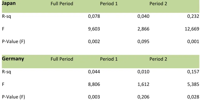
Table 2
Japan Full Period Period 1 Period 2
R-sq 0,078 0,040 0,232
F 9,603 2,866 12,669
P-Value (F) 0,002 0,095 0,001
Germany Full Period Period 1 Period 2
R-sq 0,044 0,010 0,157
F 8,806 1,612 5,385
P-Value (F) 0,003 0,206 0,028
important increase in explanatory power and suggests a strong change in the relationship between these two variables.
Turning to the results for Germany the picture repeats itself albeit not as strongly as in the case of Japan. Initially, it is interesting to note that the regression for period 1 fails to show any significant relationship between the variation in net exports and the variation in national output. This is in strong contrast to the estimation for period 2 which indicates a stronger and significant relationship between net exports and national output with a returned r-sq of 0.157 and more importantly an F-stat of 5.4 with a corresponding p-value of 0.03. Clearly, the relationship between national output and net exports is not as strong as in the case of Japan which may be due to the fact that the income balance is not included in the estimations for Germany or simply, that the relationship is not as strong.
As a final step in the empirical analysis it is worthwhile to attempt a correction of the fact that although the breaking point chosen to distinguish between periods does have an underlying merit in terms of the idea as a median age of 40 as somewhat of a watershed, it is still somewhat arbitrary. More importantly, it is clear that the results are bound to very sensitive to the choice of a breaking point even if it may be wisely chosen at the offset. In this way, the following analysis provides a number of simulations of the proposed
relationship between the variation in the external balance and the variation in national income/output. The main idea is to smooth out and essentially provide a continuous account of the relationship rather than the one above which is discrete by nature.
The approach here will still be OLS but to avoid actually estimating9 a large number of regressions it is worthwhile noting the following important results in the context of a univariate OLS framework, Gujarati (2003).
β
σ
β
σ
=
=
−
=
−
−
Consider consequently the same regression as estimated above;
α
β
= + +
Applying the three results above it is now possible to represent the evolution of the relationship between the variation of the external balance and national income as the evolution in these three variables over time. The idea is then to compute the value of these three parameters as a 10 year moving average (41 quarters/observations). This gives us 75 regressions for Japan using the data from Q1-1980 to Q4-2008 and 155 regressions for Germany where the sample size runs from Q1-1960 to Q3-2008. The idea is that this simulation should provide a stronger foundation upon which to check the robustness of the results
reported above. The results can be studied in detail in the appendix, but the two following charts for Japan and Germany respectively capture the essence of the argument (with median age to the left and the R-Sq to the right).
To the left on the graphs and depicted with the bar the median age is reported and since quarterly median ages are not reported, this time series is constructed by dividing the annual increase (or decrease) in
-0,05 0,00 0,05 0,10 0,15 0,20 0,25 0,30 30 32 34 36 38 40 42 44 Q 2 -1 9 8 0 Q 2 -1 9 8 1 Q 2 -1 9 8 2 Q 2 -1 9 8 3 Q 2 -1 9 8 4 Q 2 -1 9 8 5 Q 2 -1 9 8 6 Q 2 -1 9 8 7 Q 2 -1 9 8 8 Q 2 -1 9 8 9 Q 2 -1 9 9 0 Q 2 -1 9 9 1 Q 2 -1 9 9 2 Q 2 -1 9 9 3 Q 2 -1 9 9 4 Q 2 -1 9 9 5 Q 2 -1 9 9 6 Q 2 -1 9 9 7 Q 2 -1 9 9 8
10 Year Moving Average Median Age and R-Sq -Japan
median age R-Sq 0,000000 0,050000 0,100000 0,150000 0,200000 0,250000 0,300000 0,000 5,000 10,000 15,000 20,000 25,000 30,000 35,000 40,000 45,000 0 1 -0 1 -1 9 6 0 0 1 -0 1 -1 9 6 2 0 1 -0 1 -1 9 6 4 0 1 -0 1 -1 9 6 6 0 1 -0 1 -1 9 6 8 0 1 -0 1 -1 9 7 0 0 1 -0 1 -1 9 7 2 0 1 -0 1 -1 9 7 4 0 1 -0 1 -1 9 7 6 0 1 -0 1 -1 9 7 8 0 1 -0 1 -1 9 8 0 0 1 -0 1 -1 9 8 2 0 1 -0 1 -1 9 8 4 0 1 -0 1 -1 9 8 6 0 1 -0 1 -1 9 8 8 0 1 -0 1 -1 9 9 0 0 1 -0 1 -1 9 9 2 0 1 -0 1 -1 9 9 4 0 1 -0 1 -1 9 9 6 0 1 -0 1 -1 9 9 8
10 Year Moving Average Median Age and R-Sq - Germany
median age equally between the quarters in a given year. On the right hand side the vector of R-Sq values computed in the simulations are shown with each value corresponding to a regression with 41
observations. In terms of statistical significance, anything not including observations from 1999 and onwards is not significant (i.e. starting at 1989 in the graph) and in the case of Germany there has been three periods where the relationship between the variation in the trade balance and the variation in national output has been statistically significant; these correspond naturally to the three periods of increase seen in the graph. It is very important to note in this respect that in terms to the first two periods, the external balance of Germany was actually in a deficit and can thus hardly be claimed to constitute export reliance or dependency for that matter.
It is natural in this case to look at the trend lines which are fitted to the time series in question10 and thus essentially these two time series as a function of time. In Japan’s case the, the values for the fitted trends and their R-square values are;
= +
− = −
with the R-sq of the fitted lines with respect to time being 0.9969 and 0.6628 for “median age” and “R-SQ” respectively. For Germany we have;
= +
− = +
with the R-sq of the fitted lines equal to 0.9463 and 0.0634 for “median age” and “R-SQ” respectively.
Not surprisingly, the relationship between time and median age appears very strong which suggests a strong positive time trend for both countries in question in terms of ageing. Turning to the more interesting question of whether the computed R-sq values also contain a time trend the result seems to clearly suggest so in the context of Japan while the evidence is much less clear in a German case. Consequently, there appears to be a strong and significant positive trend in terms of the R-sq values computed from the Japanese data whereas the time trend in a German context indeed is positive albeit much weaker and for all intent and purposes not statistically significant. In Japan’s case, and using annual values, the average increase in the R-sq value measuring the relationship between the change in national income and the change of the current account has been roughly 1% per year since 1980. In the context of Germany the corresponding figure is 0.16% on average since 1960, but this figure is almost definitely not statistically significant. In this way, the results from the analysis above seem much more robust in the case of Japan than in the case of Germany.
10
Before leaving the empirical estimation, it is worthwhile noting that the robustness analysis above is bound to be quite sensitive to the fact that the sample periods differ in the two cases. Consequently, considerable stronger results would have been obtained if one had used the same sample period in for Germany as for Japan. Conversely, one would assume that had the sample period for Japan been expanded to cover the same breath of time in the case of Germany, the results would have been somewhat weaker. This
highlights the fundamental calibration issue in terms of specifying when an economy can seen to be old. In this sense, the fact that the analysis for Japan begins at a median of roughly 35 years relative to in Germany where the analysis commences when the median age is about 32-33 is not unimportant.
5.0 A Perspective on Global Capital Flows
The analysis above, if taken to heart, has clear implications for global capital flows not least in relation to the ongoing discourse and debate on global macroeconomic imbalances.
Consequently, it is worthwhile to note that the analysis above is contingent on the assumption that the extent to which an ageing economy (e.g. Germany or Japan) may develop an intertemporal preference for savings over consumption, the actual presence of an external surplus can only materialize in relation to another economy having an intertemporal preference with opposite signs; following e.g. the model in Buiter (1981). More importantly, whatever the intertemporal preference for savings and consumption may be for the collective mass of global economies, the constraint that the sum of net external position must equal zero still holds in all periods. These points direct us to a paradox or, if you will, a dilemma of important proportions in the context of the contemporary discourse on global capital flows defined as it were, by the notion of global macroeconomic imbalances.
This paradox arises as a function of the simple fact that the world is ageing and in particularly so, in an OECD context. Thus, we are moving towards a situation where a large batch of economies will age to essentially unprecedented levels and needless to say; the extent to which this is associated with a desire to export in order to maintain growth, it cannot be a strategy followed by all, or a lot, of economies at the same time. The crucial question then becomes; how will, or indeed can, the process of global ageing be transmitted to the global economy through capital flows?
As a starting point to answer this question I would like to draw the attention to comments made by two of the most prominent members of the global financial punditry in the form of US economist Paul Krugman (PK) and the Financial Times’ chief economics commentator Martin Wolf (MW). Starting with the former11 he recently pointed to the fact that external demand was instrumental in ending the slump in Japan and providing a relative bounce between 2003 and 2007. As PK further goes to argue, this may present a rather ominous outlook since the extent to which we are all, in the OECD, currently stuck in a “Japan-style” liquidity trap the way out may constitute a rather crowded route. As PK poignantly points out at the end;
And needless to say, we can’t all export ourselves out of a global slump. So, how does this end?
Krugman 2009
This is indeed a good question and MW makes a similar argument in a recent column12 where he points towards the fact that the global imbalances themselves may prove to be an impediment to a swift global recovery.
In short, if the world economy is to get through this crisis in reasonable shape, creditworthy surplus countries must expand domestic demand relative to potential output. How they achieve this outcome is up to them. But only in this way can the deficit countries realistically hope to avoid spending themselves into bankruptcy.
Martin Wolf (2008)
This is of course a very appealing proposition and also goes to heart of idea that, at least, one part of the solution of the current global crisis lies in the resolution of global macroeconomic imbalances. But prey tell, how are these surplus countries going to revert towards a growth path characterized by a more balanced external account and perhaps even an external deficit?
It is in this context that the argument presented in this paper becomes important. Consequently, there is a big risk that these surplus economies (e.g. Japan and Germany) simply will not be able to heed the call of MW. The main reason for this inability is then, in part, exactly to be found in the economic profile of a rapidly ageing economy with a median age pushing 40 year mark and beyond. Japan and Germany as well as the economies next in line to reach their age bracket cannot achieve growth based on domestic demand in a way which would allow them to suck up excess global capacity through an external deficit.
This is a very important point to stress in the context of the global economy and future contributions should attempt to shed light on the manifestation of global ageing on global capital with a specific eye to the idea that an ageing economy may develop an intertemporal preference for savings over consumption. Following this, future contributions should also seek to effectively pin down the theoretical link between ageing and (dis)saving on an aggregate macroeconomic level since it is ultimately through this that we may learn how ageing will affect open economy macroeconomics and
6.0 Conclusion
In this paper, the potential link between the reliance or dependency on exports and ageing has been investigated in the context of Germany and Japan.Two main messages should be taken away from the analysis; one theoretical and one empirical.
On the theoretical front, this paper has argued that the hypothesis of dissaving which arises in the context of a standard life cycle framework may not conform well to optimal behavior from the point of view of an individual aggregate economy. In particular, the notion that an ageing economy may come to rely on external funding to supply a deficit which arises as the supply of domestic savings decline faster than domestic investment demand seems difficult to reconcile with rational economic behavior. Once
reasonable doubt has been raised about this point, it does not take a large step to develop the idea that a
rapidly ageing economy, in an open economy context, may develop an intertemporal preference for maintaining domestic savings consistently higher than domestic investment which will, all things equal, result in an external surplus. Coupled with the notion that the economy’s ability to generate top line growth declines as a function of the process of ageing, it may generate a situation in which an economy comes to rely or perhaps even becomes dependent on external demand to generate growth in national output.
List of References
Bloom, David E; Canning, David; Fink, Günther; and Finlay, Jocelyn (2007) – Does Age Structure Forecast
Economic Growth? Harvard School of Public Health, PGDA Working Paper#20.2007
Bloom, David E; Canning, David; Fink, Günther; and Finlay, Jocelyn (2009) – The Cost of Low Fertility in
Europe, NBER Working Paper 14820
Buiter, Willem H (1981) – Time Preference and International Lending and Borrowing in an Overlapping
Generations Model, NBER Working Paper No 352
Borsch-Supan, Axel H; Alexander, Ludwig; and Krüger Dirk (2007) – Demographic Change, Relative Factor
Prices, International Capital Flows and their Differential Effects on the Welfare of Generations, NBER
Working Paper No W13185
Chow, C. Gregory (1960) – Tests of Equality Between Sets of Coefficients in Two Linear Regressions,
Econometrica vol. 28 no. 3 (1960) pp. 591-605
Cutler, David M., James M. Poterba, Louise M. Sheiner and Lawrence H. Summers (1990) – An Aging
Society: Opportunity or Challenge? Brookings Papers on Economic Activity, Vol. 1990, No. 1: 1-56
Deaton, Angus (2005) – Franco Modigliani and the Life Cycle Theory of Consumption, Research Program in
development studies and Center for Health and Wellbeing, Princeton University; the paper was presented ad the Convego Internazionale Franco Modigliani Feb. 17th-18th March 2005
Feroli, Michael (2003) – Capital Flows Among the G-7 Nations: A Demographic Perspective, Federal Reserve
Board Division of Research and Statistics
Fisher, Irvin (1930) – The Theory of Interest,
Friedman, Milton (1957) – A Theory of the Consumption Function, Princeton University Press
Gómez, Rafael & Hérnandez de Cos, Pablo (2006) – The Importance of Being Mature, The Effect of
Demographic Maturation of Global Per-Capita GDP, ECB Working Paper no. 670 August 2006
Greene, William H. (2003) – Econometric Analysis, 5th edition Prentice Hall
Gujarati, Damodar N. (2003) – Basic Econometrics 4th edition McGraw Hill
Henriksen, Esben (2002) – A Demographic Explanation of U.S. and Japanese Current Account Behavior,
Graduate School of Industrial Administration, Carnegie Mellon University
Higgins, Matthew (1998) – Demography, National Savings, and International Capital Flows, International
Economic Review, Volume 39 (1998) Issue (Month): 2 (May) pp 343-69
Malmberg, Bo and Lena, Sommestad (2000) – Four Phases of the Demographic Transition, ”Implications for
Economic and Social Development in Sweden 1820-2000” Arbetsrapport/Institut för Framtidsstudier;
Modigliani, Franco & Ando, Albert (1963) – The “Life Cycle” Hypothesis of Saving: Aggregate Implications
and Tests, The American Economic Review, vol. 53, no. 1, part 1 (Mar., 1963) pp. 55-84.
Obstfeld, Maurice & Rogoff, Kenneth (1996) – Foundations of International Macroeconomics, MIT Press
Poterba, J. (2004) – Impact of Population Ageing on Financial Markets in Developed Countries, Economic
Review 4th quarter, Federal Reserve Bank of Kansas City, pp. 43-53.
Samuelson, Paul A. (1958) – An exact consumption loan model of interest with or without the social
Appendix
Fertility and Life Expectancy
60 65 70 75 80 85 1 9 5 0 -1 9 5 5 1 9 5 5 -1 9 6 0 1 9 6 0 -1 9 6 5 1 9 6 5 -1 9 7 0 1 9 7 0 -1 9 7 5 1 9 7 5 -1 9 8 0 1 9 8 0 -1 9 8 5 1 9 8 5 -1 9 9 0 1 9 9 0 -1 9 9 5 1 9 9 5 -2 0 0 0 2 0 0 0 -2 0 0 5 2 0 0 5 -2 0 1 0 Source: UN
Life Expectancy (at birth) Germany Japan
1,1 1,2 1,3 1,4 1,5 1,6 1,7 1,8 1,9 2 2,1 2,2 2,3 1 9 7 0 1 9 7 3 1 9 7 6 1 9 7 9 1 9 8 2 1 9 8 5 1 9 8 8 1 9 9 1 1 9 9 4 1 9 9 7 2 0 0 0 2 0 0 3 2 0 0 6
Source: OECD and Nationmaster
Total Fertility Rates Japan
Ja p a n a n d G e rm a n y a s o p e n E co n o m ie s 0 0 ,0
5 0,1
0
,1
5 0,2
0
,2
5 0,3
0
,3
5 0,4
Regression results related to table 2
Japan
$ % & " ' ( ) ()*
- 0
0$12 3
0$12 3
3 3 4
5 2
6 676
0 8 %+ %+ %$
0 3 %+ %+
( %+
( %$
" & " ' ( ) ' +)*
- 0
0$12 3
0$12 3
3 3 4
5 2
6 676
0 8 %+ %+
0 3 %+ %+
( %+
( %$
, & " ' ()' ()*
- 0
0$12 3
0$12 3
3 3 4
5 2
6 676
0 8 %+ %+ %$
0 3 %+ %+
( %+
( $ $
Germany
$ % & " ) ' )- (
- 0
0$12 3
0$12 3
3 3 4
5 2
6 676
0 8
0 3
(
( %$
" & " ) ' )*
- 0
0$12 3
0$12 3
3 3 4
5 2
6 676
0 8
0 3
(
( %$
, & " )' ' )- (
- 0
0$12 3
0$12 3
3 3 4
5 2
6 676
0 8 %+ %+
0 3 %+ %+
( %+
1: 8 %$
Graphs for Robustness Results
In order to understand the numbers behind these graphs I refer to the Data CD and the tab labeled “simulation” which will give you the details on how the numbers are constructed. Essentially, these values are moving average representations (10 years) of regressions and thus attempt to catch the development of the relationship between net exports (the current account) and output growth. The regression used to do the simulation is the same univariate regression as reported above.
Japan 0 0,05 0,1 0,15 0,2 0,25 0,3 0 0,5 1 1,5 2 2,5 3 3,5 4 Q 2 -1 9 8 0 Q 2 -1 9 8 1 Q 2 -1 9 8 2 Q 2 -1 9 8 3 Q 2 -1 9 8 4 Q 2 -1 9 8 5 Q 2 -1 9 8 6 Q 2 -1 9 8 7 Q 2 -1 9 8 8 Q 2 -1 9 8 9 Q 2 -1 9 9 0 Q 2 -1 9 9 1 Q 2 -1 9 9 2 Q 2 -1 9 9 3 Q 2 -1 9 9 4 Q 2 -1 9 9 5 Q 2 -1 9 9 6 Q 2 -1 9 9 7 Q 2 -1 9 9 8
10 Year Moving Average
Beta and R-Sq -Japan Beta (10 year moving av.) R-Sq
0 0,05 0,1 0,15 0,2 0,25 0,3 0 2 4 6 8 10 12 14 16 Q 2 -1 9 8 0 Q 2 -1 9 8 1 Q 2 -1 9 8 2 Q 2 -1 9 8 3 Q 2 -1 9 8 4 Q 2 -1 9 8 5 Q 2 -1 9 8 6 Q 2 -1 9 8 7 Q 2 -1 9 8 8 Q 2 -1 9 8 9 Q 2 -1 9 9 0 Q 2 -1 9 9 1 Q 2 -1 9 9 2 Q 2 -1 9 9 3 Q 2 -1 9 9 4 Q 2 -1 9 9 5 Q 2 -1 9 9 6 Q 2 -1 9 9 7 Q 2 -1 9 9 8
10 Year Moving Average
0 0
,0
5
0
,1 0,15 0,2 0,25 0,3
0 ,0 % 0 ,5 % 1 ,0 % 1 ,5 % 2 ,0 % 2 ,5 % 3 ,0 % 3 ,5 % 4 ,0 % Q2-1980 Q2-1981 Q2-1982 Q2-1983 Q2-1984 Q2-1985 Q2-1986 Q2-1987 Q2-1988 Q2-1989 Q2-1990 Q2-1991 Q2-1992 Q2-1993 Q2-1994 Q2-1995 Q2-1996 Q2-1997 Q2-1998 1 0 Y e a r M o v in g A v e ra g e C A /G D P a n d R -S q -J a p a n C A /G D P R -S q -0 ,0 5 0 ,0 0 0 ,0 5 0 ,1 0 0 ,1 5 0 ,2 0 0 ,2 5 0 ,3 0 3
0 32 34 36 38 40 42 44
G e rm a n y 0 ,0 0 0 0 0 0 0 ,0 5 0 0 0 0 0 ,1 0 0 0 0 0 0 ,1 5 0 0 0 0 0 ,2 0 0 0 0 0 0 ,2 5 0 0 0 0 0 ,3 0 0 0 0 0 -0
,6 -0,4 -0,2 0 0,2 0,4 0,6 0,8 1
0 ,0 0 0 ,0 5 0 ,1 0 0 ,1 5 0 ,2 0 0 ,2 5 0 ,3 0 -4
% -3% -2% -1% 0% 1% 2% 3% 4% 5%