Internet network externalities

Internet network externalities

Cooper, Russel and Madden, Gary G

Macquarie University, Australia, Curtin University of Technology,

School of Economics and Finance, Perth WA 6845, Australia

2008

Online at

https://mpra.ub.uni-muenchen.de/13004/

Internet network externalities

Russel Cooper

Department of Economics Macquarie University

North Ryde, NSW 2112, Australia E-mail: rcooper@efs.mq.edu.au

Gary Madden*

Department of Economics Curtin University of Technology Perth, WA 6845, Australia E-mail: g.madden@curtin.edu.au *Corresponding author

Abstract: A driving force behind the emergence of the ‘new’ or information economy is the growth of the internet network capacity. A fundamental problem in mapping this dynamic is the lack of an acceptable theoretical framework through which to direct empirical investigations. Most of the models in the literature on network externalities have been developed in a static framework, with the externalities viewed as instantaneous or self-fulfilling. The model specified here builds on the received theory from several sources to extend these features and develops a dynamic model that is both capable of econometric estimation and which provides as an output a direct measure of the network effect. Accordingly, the main goal of this paper is to find the magnitude of the external effect on internet network growth. In addition, this paper illustrates the ability of the panel data to generate estimates of structural parameters capable of explaining internet host growth.

Keywords: information; network externalities; internet; growth.

Reference to this paper should be made as follows: Cooper, R. and Madden, G. (2008) ‘Internet network externalities’, Int. J. Management and Network Economics, Vol. 1, No. 1, pp.21–43.

Biographical notes: Russel Cooper is a Professorial Research Fellow at Macquarie University, Australia. Research interests include intertemporal optimisation models in economics, the duality theory and its applications in economics, new growth economics, inter-industry modelling, applications of rational economic modelling in specific industries, applied consumer demand studies and spatial economics. Current research projects include the estimation of cost functions, the investment decisions of high-technology firms, the investigation of network externalities in the info-communications sector, forecasting with short time series and the economic modelling of technology transfer across the digital divide.

of 78 peer-reviewed publications in these fields since 1993 and has attracted over $1M to the University for his research since 1994. In particular, he is the Chief Investigator on four Australian Research Council (ARC) Discovery Project (Large) grants since 1998. He is a Consultant to the government and a Member of the Board of Directors of the International Telecommunications Society. He is currently the Associate Editor of the International Journal of Management and Network Economics and an Editorial Board Member of The Open Communication Science Journal and the Journal of Media Economics. He is a Member of the Scientific Council of Communications and Strategies.

1 Introduction

The internet is a distribution system or conduit through which content is sent. Traditional telecommunications systems are specialised in that they (essentially) carry only two-way simultaneous voice messages along dedicated circuit-switched paths and they are not easily modified to do much else (Economides and White, 1994). What is different (and unique) about the internet network is that it is both two-way broadband and interactive. Just about any electronic signal can be sent, more or less, from anybody to anybody else (Faulhaber, 1999). Another distinguishing feature of internet traffic is that it is packet-switched, i.e., no continuous path is devoted to the delivery of a message.

Recent internet network growth has created new and expanded existing markets for broadband (bandwidth) capacity to carry two-way interactive high-speed data transfers. Accordingly, the internet has the potential to increase productivity growth and generate wealth in a variety of distinct but mutually reinforcing ways (Litan and Rivlin, 2001). Given this potential, a recent OECD (2000) finding that indicates that the European Union (EU) is lagging behind the USA in terms of internet penetration is important. That study shows, e.g., that in March 2000, there were 185 internet hosts per 1000 inhabitants in the USA compared to 41 per 1000 in the UK and 16 per 1000 in France. Further, it is suggested that internet access pricing structures may be a key factor in explaining penetration (Bourreau, 2001; Rappoport et al., 2002). A fairly natural question then for economists to consider is whether the differential rates of internet system growth is due to internet access pricing structures or, more fundamentally, growth generated by direct network externalities after a critical system mass is achieved.

Economides and Himmelberg (1995) refine the notion of critical mass as the smallest size network that can be sustained in equilibrium. They argue that when the critical mass is substantial, market coverage will not be achieved – either the market does not exist or it is of insufficient coverage.2 Accordingly, consumer willingness to adopt internet service is an increasing function of network size (Shy, 2001). The existence of network externalities in a dynamic setting increases the speed at which market demand grows in the presence of a downward trend for industry marginal cost. Given the possible existence of a network externality for internet connection (and e-commerce), estimates of the size of the network effect are critical for forecasting demand and in network planning. Accordingly, a model is developed here to describe the global internet market growth that provides a detailed analysis of the nature of the externality.

Bensaid and Lesne (1996) argue that most network externality models are developed in a static framework, with externalities viewed as either instantaneous or self-fulfilling. An Economides (1996) dynamic ‘macro’ approach is employed here to analyse the role network externalities have in explaining internet system growth in a continuous-time setting. The ‘macro’ approach simply assumes network externalities exist and attempts to model their consequences.3 Further, here the notion of network externality is broadened to include those due to producer activity. Interaction between agents’ (consumers’ and firms’) decisions is considered by a representative agent model in which sustained growth is the result of positive externalities from investment in network input n. Agents are linked through income flows and endogenous growth in the internet network occurs through the inclusion of a network externality in the production argument in the ‘old economy’ firms’ production function and also in the consumer’s instantaneous utility function. The system is stochastic because the return to the representative consumer from Applications Sector (AS) investment is uncertain. The stochastic income specification leads to a stochastic inter-temporal optimisation problem. The resultant solution provides an optimised network growth equation for estimation. The model is estimated on cross-country panel data to yield a direct measure of the strength of the network effect.

The paper is organised as follows. Section 2 specifies a model to examine internet network growth that incorporates a network externality. In Section 3 data and variables used in estimation are presented and described. The empirical modelling strategy is explained in Section 4, and estimates of network externalities are reported. Concluding remarks and policy implications are provided in Section 5.

2 A dynamic model of internet network growth

2.1 Network production externalities

Let F(v,n,n*) denote the production function of a representative firm where v is either an aggregate non-network input or a vector of non-network inputs, e.g., labour and non-network capital. Let n* represent a network externality generated through productive activity. This argument allows ‘endogenous growth’ to occur in the network growth equation, viz., the production function exhibits decreasing returns in n (from the perspective of the firm) and increasing returns when n is equated to n* post-optimisation. That is, during optimisation n* is treated by the firm as exogenous, and post-optimisation

n* is equated to n when model equations are derived. Thus positive externalities arise from network capital and are a source of increasing returns in production. Let w represent the price of variable inputs. Illustration of the ‘optimising out’ process is provided for the case where v is a variable input. Consider the production function:

1

( , , *) (1 *)

F v n n =v nα −α +n β (1)

and the instantaneous variable profit function (conditional on network size, n):

( , , *)w n n max_v F v n n( , , *) wv.

Π = 〈 − 〉 (2)

The solution for optimal v is:

1 /(1 ) 1 /(1 ) /(1 )

ˆ (1 *)

v=α −α w− −α +n β −α n (3)

where the linearity of ˆv in n follows from the linear homogeneity of the production function in (v,n).

Conditional on the n, optimised output can then be constructed as a function of input prices:

/(1 ) /(1 ) /(1 )

ˆ ( , , *) (1 *) .

F w n n =αα −αw−α −α +n β −α n (4)

Further, the linearity of optimised output in n, i.e., from the point of view of the firm’s optimisation, without internalising the externality, is emphasised by writing:

ˆ ( , , *) ( , *)

F w n n =R w n n (5)

where R(w,n*) is the return per unit of network capital:

/(1 ) /(1 ) /(1 )

( , *) (1 *) .

R w n =αα −α w−α −α +n β −α (6)

∂R(w,n*)/∂n* > 0 indicates the production network externality directly augments the return per unit of network capital or interest rate in this stylised model.

2.2 Network consumption externalities

Internet network externalities can also arise through consumption. Let U(c,n*) denote the instantaneous utility function of a representative consumer where c is real total consumption and n* is the current network size for an average firm (which is outside the control of the consumer). The point of departure here is the standard iso-elastic utility specification that emphasises the importance of the inter-temporal elasticity of substitution (IES= –∂lnc/∂lnUc). Temporarily setting aside the network effect, specify

( , ) .

U ci =cγ (7)

The IES for (7) is:

1 /(1 ),

IES= −γ (8)

where –∞ < γ < 1. The IES indicates the willingness of a consumer to forego current consumption in favour of current saving and greater discounted future utility, viz., consumer flexibility. Here the network consumption externality is introduced through the IES, i.e., as income is received from n* and as consumer flexibility might realistically be income dependent, it seems reasonable to suspect the IES is affected by n*. The specification adopted here is:

1 2

1 *

.

1 * 1 *

n IES

n n

θ ⎡ ⎤ θ ⎡ ⎤ = _{⎢ ⎥}+ _{⎢ ⎥}

+ +

⎣ ⎦ ⎣ ⎦ (9)

In Equation (9) the IES ranges in value from θ1 when there is no network rollout (n* = 0) and asymptotes to θ2 as the network expands indefinitely (n* →∞). The IES is increasing in n* if θ2 > θ1, viz., the consumer becomes more flexible. Accordingly, the utility function incorporating network externality effects is written as a function of network size G(n*):

( *)

( , *) G n

U c n =c (10)

where since IES= 1/[1–G(n*)] or G(n*) = 1–1/IES, and with the IES given by (9), G(n*) is specified:

1 2

1

( *) 1 .

1 *

1 * 1 *

G n

n

n n

θ θ

= −

⎡ ⎤₊ ⎡ ⎤ ⎢ ₊ ⎥ ⎢ ₊ ⎥

⎣ ⎦ ⎣ ⎦

(11)

2.3 Income flows

The old economy firm produced output through Equation (5). This output is a source of income to the owners of the firm – the consumers. Income is also derived from a stochastic return to consumers from AS (new economy) investment obtained by selling x

of the network n. In doing so the consumer foregoes a ‘sure’ rate of return R(w,n*)xdt for receipt of risky return xdq/q. While uncertainty of income flow is expected for both new and old economy firms – it seems reasonable to assume that new economy firm returns are the more uncertain. To focus attention, uncertainty is isolated to the returns of the new economy firm. Here the risky asset is assumed to pay no dividend and provide only a capital gain or loss. The resulting flow of consumer income from production and investment sources is:

( , *) [ / ( , *) ]

dy=R w n ndt+ dq q−R w n dt x (12)

where the price of the risky asset, q, is modelled as following a geometric Brownian motion with drift µq and volatility σq:

q q q

dq=µqdt+σ qdz (13)

2.4 Expenditure

An alternative to consumption is the retention of earnings by the firm, which are employed to extend the network. Consequently, network expansion is stochastic and so the demand side of the income identity is:

,

dy=cdt+pdn (14)

where the network access price p converts the value of the network extension into units of the consumption good.

2.5 Optimisation model

For the stochastic income specification Equation (12) through Equation (14), the representative consumer’s inter-temporal optimisation problem is:

0 0 0 { ( ), ( )} 0 0

( , , ) max t ( ( ), * ( ))

c t x t

J n p w E e δU c t n t dt

∞ −

=

∫

subject to:

( , *) / ( , *)

R w n n c dq q R w n dt

dn dt x

p p

⎡ − ⎤ ⎡ − ⎤

=_{⎢ ⎥} +_{⎢ ⎥}

⎣ ⎦ ⎣ ⎦ (16)

q q q

dq=µqdt+σ qdz (17)

p p p

dp=µ pdt+σ pdz (18)

w w w

dw=µ wdt+σ wdz (19)

* ( ) ( ), [0, )

n t =n t t∈ ∞ (20)

0 0 0

(0) , (0) , (0) .

n =n p =p w =w (21)

2.6 Optimised network growth equation

Combining Equation (16) and Equation (17) the network growth equation can be characterised as a diffusion of the form:

( , *) [ ( , *)]

.

q q

q

R w n n R w n x c x

dn dt dz

p p

µ σ

+ − −

⎧ ⎫

=⎨ ⎬ +

⎩ ⎭ (22)

Due to the time-autonomous nature of Equation (15), the solutions for c and x may be obtained in feedback or synthesised form, expressing the controls as a function of the current values of the states of n, p and w. To describe the solution, it is useful to define the latent variables:

( , *)

r=R w n (23)

and

1 /[1 ( *)],

interpretable as the interest rate and the IES, respectively. Also note that n=n* in the optimised model.5 Further, Cooper et al. (1995) show optimal c can be written:

2 2 1

ˆ [1 ] ( ) /

2 q q

c=⎧_⎨hδ + −h r_⎢⎡ + hµ −r σ _⎥⎤_⎬⎫n

⎣ ⎦

⎩ ⎭ (25)

and optimal x as:

2

ˆ q .

q

r

x h µ n

σ ⎡ − ⎤ = ⎢ ⎥ ⎢ ⎥

⎣ ⎦ (26)

Utilising the synthesised solutions Equation (25) and Equation (26), and substituting into (22), provides the optimal network diffusion:

2 2

1

[ 1]( ) /

2 q q

q

q q

r h r _r

dn h ndt h ndz

p p

δ µ σ _µ

σ ⎧ _{− + + −} ⎫

⎧ − ⎫

⎪ ⎪ _{⎪ ⎪}

= ⎨ ⎬ + ⎨ ⎬

⎪ ⎪

⎪ ⎪ ⎩ ⎭

⎩ ⎭

(27)

where, in view of the specifications of technology and preferences, and setting n=n*:

/(1 ) /(1 ) /(1 )

[1 ]

r=αα −α w−α −α +nβ −α (28)

and

1 2

1

.

1 1

n h

n n

θ ⎡ ⎤ θ ⎡ ⎤ = _{⎢ ⎥}+ _{⎢ ⎥}

+ +

⎣ ⎦ ⎣ ⎦ (29)

3 Data and variables

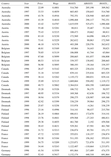
Mean, standard deviation, minimum and maximum values for HOST, ∆HOST, PRICE and WAGE are reported in Table 1. Host numbers (HOST) range in value from less than four thousand (Luxembourg) to in excess of 80 million (US). The mean addition to the HOST count (∆HOST), across both countries and time, is almost 800 000. Eleven countries recorded declines in host numbers, with the largest decline in France (2000).10 PRICE, the listed price of dominant ISP and PSTN carriers, ranges in value from USD18.96 (US) to USD291.43 (Mexico). Average WAGE compensation is 48% of GDP and reflects considerable variation across the sample from 26% (Turkey) to 61% (Switzerland).

Table 1 Summary statistics 1996–2000

Variable Mean Standard deviation Minimum Maximum

Complete sample

HOSTS 2 043 942 9 130 292 3518 80 566 944

∆HOSTS 737 982 3 397 557 –110 664 27 390 988

PRICE 53.05 33.73 18.96 291.43

WAGE 0.48 0.08 0.26 0.61

Sample with Mexico and Turkey excluded

HOSTS 2 209 516 9 504 014 3518 80 566 944

∆HOSTS 796 852 3 537 170 –110 664 27 390 988

PRICE 48.41 20.36 18.96 135.69

WAGE 0.50 0.06 0.32 0.61

Notes: HOST is host numbers. ∆HOST = HOSTt – HOSTt–1. PRICE is the real price of internet access in USD purchasing power parity.

4 Model estimation

4.1 Functional form specification

The network growth equation was derived in Section 2 in continuous time as Equation (27) to Equation (29). Converting to discrete time, let dt= 1, dn=nt – nt–1=∆nt and dzq=

εq ~ N(0,1). The estimating form becomes:

( )

_[

_]

/ 1 /(1 ) 1 1

1 2

1 1 1

1 1

1 2 1 2

1 1 1 1

/(1 )

1 1

1 1

1 1 1

(1 ) (1 )

2 1 1 1 1

(

t t

t t

t t t t

t t

t t t t

q

w n

n n

n n n p

n n

n n n n

w

β α

α α α α

α α

α δ

θ θ

θ θ θ θ

µ α − − − − − − − − − − − − − − − − ⎧ ⎡ ⎤ ⎡ ⎤⎫ + − ∆ ₌⎪ ₊ ⎪ ⎨ ⎢ ₊ ⎥ ⎢ ₊ ⎥⎬ ⎪ ⎣ ⎦ ⎣ ⎦⎪ ⎩ ⎭ ⎧ ⎡ ⎤ ⎡ ⎤⎫ ⎧ ⎡ ⎤ ⎡ ⎤⎫ ⎪ ⎪ ⎪ ⎪ + ⎨ ⎢ ₊ ⎥+ ⎢ ₊ ⎥⎬ ⎨ + ⎢ ₊ ⎥+ + ⎢ ₊ ⎥⎬ ⎪ ⎣ ⎦ ⎣ ⎦⎪ ⎪ ⎣ ⎦ ⎣ ⎦⎪ ⎩ ⎭ ⎩ ⎭ − ×

[

]

/(1 ) 2

with error term:

/(1 ) /(1 ) /(1 ) 1 1

, 1 2 ,

1 1

[1 ]

1

1 1

q t t

t

n t q t

t t t q

w n

n

n n p

α α α α β α

µ α

ε θ θ ε

σ − − − − − − − − ⎡ ⎤ ⎧ ⎡ ⎤ ⎡ ⎤⎫ − + ⎪ ⎪ =⎨ ⎢ ₊ ⎥+ ⎢ ₊ ⎥⎬⎢ ⎥ ⎪ ⎣ ⎦ ⎣ ⎦⎪ ⎢ ⎥

⎩ ⎭ ⎣ ⎦ (31)

It will prove useful to identify the components of Equation (30) that have direct economic interpretation. They are, the inter-temporal elasticity of substitution:

1 1 2 1 1 1 , 1 1 t t t n IES h n n

θ θ −

− −

⎧ ⎡ ⎤ ⎡ ⎤⎫

⎪ ⎪

= =⎨ ⎢ ₊ ⎥+ ⎢ ₊ ⎥⎬ ⎪ ⎣ ⎦ ⎣ ⎦⎪

⎩ ⎭ (32)

the ‘interest rate’ (or rate of return to the network as a productive resource), r: /(1 ) /(1 ) /(1 )

1

[1 ]

t t

r=αα −α w−α −α +n₋ β −α (33)

and the Relative Risk Premium (RRP), defined as the normalised equity premium, (µq – r)/σ relative to network access price, p:

/ .

q q

r

RRP µ p

σ ⎡ − ⎤ = ⎢ ⎥ ⎢ ⎥

⎣ ⎦ (34)

Potential heteroscedasticity is implied by Equation (31). The scale factor attached to the random error εq,t in (31) may be summarised, in view of Equation (32) and Equation (34),

as IES×RRP. This scale factor is itself a stochastic process and contains error variation that is partly predetermined (due to nt–1) and partly currently determined (due to wt and

pt). In addition, wt and pt contain partly systematic variation (since they have drifts µw and

µp) and partly random variation (in view of their specification as stochastic processes,

i.e., Equation (18) and Equation (19)). While a weighted correction procedure could be applied if all variation were predetermined or systematic, the idea of giving observations different weights because of random variation is problematic since it could induce inconsistency. An alternative approach is to note that the offending term in Equation (31),

viz., h(µq –r)/(pσq) has a drift that, though complicated, may be derived from the

underlying stochastic processes for n, p and w by application of Ito’s Lemma. Borrowing methodology from finance theory, there exist synthetic probabilities which would force this complex drift to zero, so that the offending scale factor in Equation (31), while not a constant, could at least be modelled as a martingale under the synthetic probability measure. Here it is proposed to find maximum likelihood estimates for this case. This seems more acceptable than attempting to convert the scale factor to a constant when it contains random variation.

To employ the proposed correction procedure, a variable parameter specification for components of r, h, µq and σq where they appear in Equation (30) is utilised. This may

be interpreted as indirectly estimating probabilities associated with realisations of

[

]

1 1

1, 2

1 1 1

1 1

1, 2 1, 2

1 1 1 1

1 1

1 1

1 1 1

(1 ) (1 )

2 1 1 1 1

(

c t t t

t t

t

t t t t

t t

t t

t t t t

t c t

A T w n

n n

n n n p

n n

n n n n

A T w

β α

α α _δ

θ θ

θ θ θ θ

µ − − − − − − − − − − − − − − ⎧ ⎡ ⎤ ⎡ ⎤⎫ + − ∆ ₌⎪ ₊ ⎪ ⎨ ⎢ ₊ ⎥ ⎢ ₊ ⎥⎬ ⎪ ⎣ ⎦ ⎣ ⎦⎪ ⎩ ⎭ ⎧ ⎡ ⎤ ⎡ ⎤⎫ ⎧ ⎡ ⎤ ⎡ ⎤⎫ ⎪ ⎪ ⎪ ⎪ + _{⎨ ⎢ ⎥}+ _{⎢ ⎥⎬ ⎨} + _{⎢ ⎥}+ + _{⎢ ⎥⎬} + + + + ⎪ ⎣ ⎦ ⎣ ⎦⎪ ⎪ ⎣ ⎦ ⎣ ⎦⎪ ⎩ ⎭ ⎩ ⎭ − ×

[

]

/(1 ) 2

1 2 1 ) t t t t t n p β α α α ε σ − − − − + + (35)

where it is now assumed, as part of a method which employs a variable parameter specification to choose parameter estimates and indirectly generate probabilities for realisations of IES×RRP most compatible with this assumption, that 2

(0, ).

t IID N ε

ε _∼ σ

Other adjustments to Equation (30), contained in Equation (35), include subsuming the constant parameter function αα/(1–α) into the production function ‘intercept’ term A. The adjusted intercept is specified as the product of:

23 1 0 j j j c d c a

A =α +α e∑= ₍₃₆₎

and

2 2

( 1) ( 1) ( 1) ( 1) 0

/(1 )

bt ct bt ct

t a

T =τ +eτ − +τ − +τ eτ − +τ − (37)

where the cj and dj are country parameters and indicator variables (j= 1,…,23),

respectively. After a grid search, αaand α0 are pre-set at αa= 0.1 and α0= 0.01, and τa

and τ0 are pre-set at τa= 0.01 and τ0= 19. The remaining parameters, cj in the case of the

country scale factor Ac, and τb and τc in the case of the time scale factor Tt, are freely

estimated in the non-linear maximum likelihood estimation routine.

Further, θ1, µq and σq are specified as time varying, and are denoted by θ1,t, µt and σt,

respectively, as: 1 1 1, 0 1 , c US t t t c US

t

n n

n

θ θ θ − −

− ⎡ − ⎤

= _{+ ⎢ ⎥}

⎣ ⎦ (38)

2 2

( 1) ( 1) ( 1) ( 1) 0

/(1 )

bt ct bt ct

t a e e

µ µ µ µ

µ ₌µ ₊ − + − ₊µ − + −

(39)

and

2 2

( 1) ( 1) ( 1) ( 1) 0

/(1 ).

bt ct bt ct

t a e e

σ σ σ σ

σ ₌σ ₊ − + − ₊σ − + −

(40)

Following a grid search, parameter settings µa= 0.01, µ0= 4, σa= 0.05 and σ0= 29, are imposed. Remaining parameters (θ0, θ c,µb,µc, σb and σc) are freely estimated.

1

0.02 1

[1 ]

2

t t

t t t t t

t t

n r

IES IES IES RRP

n₋ p ε

∆ −

= + + + (41)

where IESt, RRPt, and rt are respectively:

1 1 1

0 2

1 1 1

0.5 1

,

1 0.5 1 0.5

c US W

t t t

t c US W W

t t t

n n n

IES

n n n

θ θ − − θ −

− − − ⎧ ⎡ − ⎤ ⎡⎫ ⎤ ⎡ ⎤ ⎪ ⎪ =_⎨ + _{⎢ ⎥ ⎢⎬ ⎥}+ _{⎢ ⎥} + + ⎪ ⎣ ⎦ ⎣⎪ ⎦ ⎣ ⎦

⎩ ⎭ (42)

2

2

2

2 2 ( 1) ( 1)

( 1) ( 1)

2 ( 1) ( 1)

( 1) ( 1) 0.01 1 4 0.05 1 29 b c b c b c b c t t t t t t t t

t _{t t}

e r e RRP e p e µ µ µ µ σ σ σ σ − + − − + − − + − − + − ⎛ ⎞ + − ⎜ ⎟ ⎜ ₊ ⎟ ⎝ ⎠ = ⎛ ⎞ + ⎜ ⎟ ⎜ ₊ ⎟ ⎝ ⎠ (43) and 23 2 1 2 ( 1) ( 1)

/(1 ) ( 1) ( 1)

/(1 ) /(1 )

1 1

0.1 0.01 0.01 1 19

[1 ] [1 (1 )] .

b c j j j b c W C t t c d

t _{t t} t

W c

t US t US

e

r e w

e

n d n d

τ τ

α α

τ τ

β α β α

= − + − − − − + − − − − − ⎡ _∑ ⎤_{⎡ ⎤} ⎢ ⎥ =_⎢ + _⎥⎢ + ⎥ + ⎢ ⎥ ⎣ ⎦ ⎣ ⎦ × + + − (44)

Network measures are constructed from internet host numbers by applying the rule:

1 0 1 0 , c c c t t c HOST HOST n HOST − − − =

where t= 1,…,5, c= 1,…,23, with 0 denoting year 1995.

4.2 Variable coefficient commentary

Before proceeding, an interpretation for the variable parameter specifications is provided. By construction, c₁ 0

t

n₋ = for t= 1. At t= 1 the interest rate applicable to holding network stock is:

23

1 /(1 )

1 0.1 0.01 0.06 1

j j j

c d

r e= w−α −α

⎡ _∑ ⎤

⎢ ⎥

= +

⎢ ⎥

⎣ ⎦

and variations in the interest rate cross country in the initial period reflects real wage conditions, differences in initial technology and network externality effects, all of which are captured by the cj.

In this specification, the technology parameter Tt takes the value T1= 0.06 for all countries at t= 1, 1996, and acts as a normalising constant. The specification:

2

2 ( 1) ( 1)

( 1) ( 1) 0.01

1 19

b c

b c

t t

t _{t t}

allows for non-monotonic behaviour of network stock efficiency in production, with common country behaviour determined by the freely estimated parameters τb and τc.

When τb(t – 1) +τc(t – 1)

2

takes a large negative value, Tt will tend to 0.01, the imposed

lower bound on Tt. In this specification, Tt can rise above its value at T1, but just. The upper bound of 0.0626 is imposed by the scaling constant value of τ0= 19. Based on similar reasoning, the remaining constrained non-linear variable parameter functions are described below.

The country-specific effect: 23

1 0.1 0.01

j j j

c d c

A = + e∑=

has a lower bound of 0.1, but no upper bound. An estimated coefficient of –91.381 for Greece implies the lower bound is binding. Other countries are not affected. An estimated value of cj= 3 suggests a corresponding parameter value of Ac= 0.3.

The expected return on the risky AS investment is modelled as: 2

2 ( 1) ( 1)

( 1) ( 1)

0.01 .

1 4

b c

b c

t t

t _{t t}

e

e

µ µ

µ µ

µ − + −

− + − = +

+

This specification forces µ1= 0.21 but allows µt to vary from 0.01 to 0.26, with values

dependent on the freely estimated parameters µb and µc. In estimation neither bound

is binding.

The volatility of risky AS investment is modelled as: 2

2 ( 1) ( 1)

( 1) ( 1)

0.05 .

1 29

b c

b c

t t

t _{t t}

e

e

σ σ

σ σ

σ = + − +_{− +}− ₋ +

This specification has a lower bound of 0.05 for σt. It also forces an initial value of

σ1= 0.083 and has an upper bound of 0.0845. σt is constrained to begin near its upper

bound. In estimation, σt fell to the lower bound by the latter part of the sample.

These variable parameter specifications capture the fall in the expected return on the AS risky investment mid-sample, making some allowance for the Asian financial crisis and world financial conditions more generally. Additionally, from an econometric point of view, the accompanying but lesser fall in volatility leads to a reduced, though substantial, fall in the RRP, countervailing a substantial rise in the IES and providing some support for the approach that treats IES×RRP as a martingale.

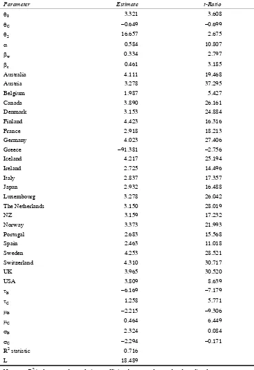
4.3 Maximum likelihood estimates

Non-linear maximum likelihood estimation of Equation (41) is performed using SHAZAM Version 8 (White, 1997). Parameter estimates and asymptotic t-statistics are presented in Table 2. The key results concern parameters associated with consumption and production network externalities. Consumption externalities are measured through the parameters θ0, θc and θ2. The non-US θC is estimated as economically small in

Table 2 Estimation results

Parameter Estimate t-Ratio

θ0 3.321 3.608

θC –0.649 –0.699

θ2 16.657 2.675

α 0.584 10.807

βw 0.334 2.797

βc 0.461 3.185

Australia 4.111 19.468

Austria 3.278 37.295

Belgium 1.987 5.427

Canada 3.890 26.161

Denmark 3.153 24.884

Finland 4.423 16.316

France 2.918 18.213

Germany 4.023 27.406

Greece –91.381 –2.756

Iceland 4.217 25.194

Ireland 2.725 14.496

Italy 2.837 17.357

Japan 2.932 16.488

Luxembourg 3.278 26.042

The Netherlands 3.150 28.019

NZ 3.159 17.232

Norway 3.373 21.993

Portugal 2.683 15.568

Spain 2.463 11.018

Sweden 4.253 28.521

Switzerland 4.310 30.717

UK 3.965 30.520

USA 3.809 8.639

τB –6.169 –7.179

τC 1.258 5.771

µB –2.215 –9.306

µC 0.464 6.449

σB 2.324 0.084

σC –2.294 –0.171

R2 statistic 0.716

L 18.489

Turning to the evidence concerning production externalities, the crucial parameters are βw

for externalities related to the size of the world network estimated at 0.334 and, βc for

externalities related to the size of specific country networks and estimated at 0.461.12 The results imply effective increasing returns to scale due to the externality of 1.334 for the US (with the world network size providing the externality) and 1.461 for other countries (with the size of the country-specific stock providing the externality).

An ancillary production function parameter is α. Estimated at 0.584, this indicates the variable factor input share of output income is 58%. Remaining parameter estimates control for country-specific effects in technology, the extent of externalities prior to 1996, for variation in the normalised risk premium and the returns to AS investment over time. Generally, these results indicate the importance of allowing for these variations in the pooled data set.

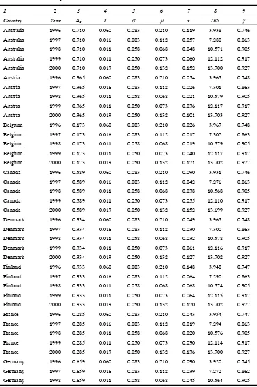
Table 3 reports variable parameter estimates and other functions that vary cross-country or time. Column (3) and Column (4) labelled AC and T, respectively,

provide estimates of the country-specific component and time-specific component that together define the scale factor for the interest rate, viz., ACTt in the expression for rt:

/(1 ) /(1 )

/(1 )

1 1

[1 W ]W [1 c (1 )]c .

t C t t t USA t USA

r =A T w−α −α +n d₋ β −α +n₋ −d β −α (45)

The interest rate, constructed according to Equation (45), is given in Column (7) of Table 3. Column (5) and Column (6) report the remaining variable parameter components of the normalised risk premium, viz., σ and µ. Comparison of Column (6) and Column (7) shows the risk premium is positive for most countries and time periods, with negative values reported for seven countries, and all in the final time period. Preliminary grid searches for economically sensible values of parameters controlling upper and lower limits on the allowable variation in estimates of Tt, µt and σt, and a lower limit for AC

are based on minimising the number of violations of non-positive risk premiums. Given these pre-set values, maximum likelihood estimation proceeded on the basis of generation of a minimal number of these economically problematic results. Column (8) reports the calculated IES values. In particular, the IES is rising through time to near its upper bound, implying that benefits from increased network size will be lower on further network expansion.

Table 3 Variable parameter estimates

1 2 3 4 5 6 7 8 9

Country Year AC T σ µ r IES γ

Australia 1996 0.710 0.060 0.083 0.210 0.119 3.938 0.746

Australia 1997 0.710 0.016 0.083 0.112 0.057 7.280 0.863

Australia 1998 0.710 0.011 0.058 0.068 0.048 10.571 0.905

Australia 1999 0.710 0.011 0.050 0.073 0.060 12.112 0.917

Australia 2000 0.710 0.019 0.050 0.132 0.152 13.700 0.927

Austria 1996 0.365 0.060 0.083 0.210 0.054 3.965 0.748

Austria 1997 0.365 0.016 0.083 0.112 0.026 7.301 0.863

Austria 1998 0.365 0.011 0.058 0.068 0.021 10.579 0.905

Austria 1999 0.365 0.011 0.050 0.073 0.036 12.117 0.917

Austria 2000 0.365 0.019 0.050 0.132 0.101 13.703 0.927

Belgium 1996 0.173 0.060 0.083 0.210 0.026 3.967 0.748

Belgium 1997 0.173 0.016 0.083 0.112 0.017 7.302 0.863

Belgium 1998 0.173 0.011 0.058 0.068 0.019 10.579 0.905

Belgium 1999 0.173 0.011 0.050 0.073 0.040 12.117 0.917

Belgium 2000 0.173 0.019 0.050 0.132 0.121 13.702 0.927

Canada 1996 0.589 0.060 0.083 0.210 0.090 3.931 0.746

Canada 1997 0.589 0.016 0.083 0.112 0.042 7.276 0.863

Canada 1998 0.589 0.011 0.058 0.068 0.038 10.568 0.905

Canada 1999 0.589 0.011 0.050 0.073 0.055 12.110 0.917

Canada 2000 0.589 0.019 0.050 0.132 0.152 13.699 0.927

Denmark 1996 0.334 0.060 0.083 0.210 0.049 3.965 0.748

Denmark 1997 0.334 0.016 0.083 0.112 0.030 7.300 0.863

Denmark 1998 0.334 0.011 0.058 0.068 0.032 10.578 0.905

Denmark 1999 0.334 0.011 0.050 0.073 0.061 12.116 0.917

Denmark 2000 0.334 0.019 0.050 0.132 0.127 13.702 0.927

Finland 1996 0.933 0.060 0.083 0.210 0.148 3.948 0.747

Finland 1997 0.933 0.016 0.083 0.112 0.064 7.290 0.863

Finland 1998 0.933 0.011 0.058 0.068 0.068 10.574 0.905

Finland 1999 0.933 0.011 0.050 0.073 0.064 12.115 0.917

Finland 2000 0.933 0.019 0.050 0.132 0.120 13.702 0.927

France 1996 0.285 0.060 0.083 0.210 0.043 3.954 0.747

France 1997 0.285 0.016 0.083 0.112 0.019 7.294 0.863

France 1998 0.285 0.011 0.058 0.068 0.020 10.576 0.905

France 1999 0.285 0.011 0.050 0.073 0.030 12.114 0.917

France 2000 0.285 0.019 0.050 0.132 0.136 13.700 0.927

Germany 1996 0.659 0.060 0.083 0.210 0.090 3.920 0.745

Germany 1997 0.659 0.016 0.083 0.112 0.039 7.272 0.862

Table 3 Variable parameter estimates (continued)

1 2 3 4 5 6 7 8 9

Country Year AC T σ µ r IES γ

Germany 1999 0.659 0.011 0.050 0.073 0.059 12.107 0.917

Germany 2000 0.659 0.019 0.050 0.132 0.118 13.699 0.927

Greece 1996 0.100 0.060 0.083 0.210 0.030 3.970 0.748

Greece 1997 0.100 0.016 0.083 0.112 0.018 7.304 0.863

Greece 1998 0.100 0.011 0.058 0.068 0.020 10.581 0.905

Greece 1999 0.100 0.011 0.050 0.073 0.038 12.118 0.917

Greece 2000 0.100 0.019 0.050 0.132 0.105 13.703 0.927

Iceland 1996 0.778 0.060 0.083 0.210 0.120 3.970 0.748

Iceland 1997 0.778 0.016 0.083 0.112 0.049 7.304 0.863

Iceland 1998 0.778 0.011 0.058 0.068 0.050 10.581 0.905

Iceland 1999 0.778 0.011 0.050 0.073 0.069 12.118 0.917

Iceland 2000 0.778 0.019 0.050 0.132 0.145 13.703 0.927

Ireland 1996 0.253 0.060 0.083 0.210 0.047 3.969 0.748

Ireland 1997 0.253 0.016 0.083 0.112 0.030 7.304 0.863

Ireland 1998 0.253 0.011 0.058 0.068 0.032 10.580 0.905

Ireland 1999 0.253 0.011 0.050 0.073 0.046 12.118 0.917

Ireland 2000 0.253 0.019 0.050 0.132 0.099 13.703 0.927

Italy 1996 0.271 0.060 0.083 0.210 0.054 3.963 0.748

Italy 1997 0.271 0.016 0.083 0.112 0.031 7.298 0.863

Italy 1998 0.271 0.011 0.058 0.068 0.039 10.577 0.905

Italy 1999 0.271 0.011 0.050 0.073 0.062 12.115 0.917

Italy 2000 0.271 0.019 0.050 0.132 0.084 13.703 0.927

Japan 1996 0.288 0.060 0.083 0.210 0.040 3.942 0.746

Japan 1997 0.288 0.016 0.083 0.112 0.033 7.270 0.862

Japan 1998 0.288 0.011 0.058 0.068 0.035 10.563 0.905

Japan 1999 0.288 0.011 0.050 0.073 0.053 12.106 0.917

Japan 2000 0.288 0.019 0.050 0.132 0.152 13.696 0.927

Luxembourg 1996 0.365 0.060 0.083 0.210 0.053 3.970 0.748

Luxembourg 1997 0.365 0.016 0.083 0.112 0.031 7.305 0.863

Table 3 Variable parameter estimates (continued)

1 2 3 4 5 6 7 8 9

Country Year AC T σ µ r IES γ

NZ 1996 0.336 0.060 0.083 0.210 0.064 3.965 0.748

NZ 1997 0.336 0.016 0.083 0.112 0.029 7.301 0.863

NZ 1998 0.336 0.011 0.058 0.068 0.041 10.578 0.905

NZ 1999 0.336 0.011 0.050 0.073 0.032 12.117 0.917

NZ 2000 0.336 0.019 0.050 0.132 0.119 13.703 0.927

Norway 1996 0.392 0.060 0.083 0.210 0.070 3.962 0.748

Norway 1997 0.392 0.016 0.083 0.112 0.035 7.298 0.863

Norway 1998 0.392 0.011 0.058 0.068 0.044 10.577 0.905

Norway 1999 0.392 0.011 0.050 0.073 0.049 12.116 0.917

Norway 2000 0.392 0.019 0.050 0.132 0.143 13.702 0.927

Portugal 1996 0.246 0.060 0.083 0.210 0.048 3.969 0.748

Portugal 1997 0.246 0.016 0.083 0.112 0.028 7.304 0.863

Portugal 1998 0.246 0.011 0.058 0.068 0.034 10.580 0.905

Portugal 1999 0.246 0.011 0.050 0.073 0.049 12.118 0.917

Portugal 2000 0.246 0.019 0.050 0.132 0.121 13.703 0.927

Spain 1996 0.217 0.060 0.083 0.210 0.032 3.965 0.748

Spain 1997 0.217 0.016 0.083 0.112 0.023 7.299 0.863

Spain 1998 0.217 0.011 0.058 0.068 0.027 10.578 0.905

Spain 1999 0.217 0.011 0.050 0.073 0.044 12.116 0.917

Spain 2000 0.217 0.019 0.050 0.132 0.123 13.702 0.927

Sweden 1996 0.803 0.060 0.083 0.210 0.101 3.955 0.747

Sweden 1997 0.803 0.016 0.083 0.112 0.051 7.294 0.863

Sweden 1998 0.803 0.011 0.058 0.068 0.051 10.576 0.905

Sweden 1999 0.803 0.011 0.050 0.073 0.056 12.115 0.917

Sweden 2000 0.803 0.019 0.050 0.132 0.141 13.702 0.927

Switzerland 1996 0.845 0.060 0.083 0.210 0.103 3.962 0.748 Switzerland 1997 0.845 0.016 0.083 0.112 0.049 7.299 0.863 Switzerland 1998 0.845 0.011 0.058 0.068 0.047 10.578 0.905 Switzerland 1999 0.845 0.011 0.050 0.073 0.064 12.117 0.917 Switzerland 2000 0.845 0.019 0.050 0.132 0.127 13.703 0.927

UK 1996 0.627 0.060 0.083 0.210 0.090 3.924 0.745

UK 1997 0.627 0.016 0.083 0.112 0.043 7.271 0.862

UK 1998 0.627 0.011 0.058 0.068 0.039 10.566 0.905

UK 1999 0.627 0.011 0.050 0.073 0.058 12.107 0.917

UK 2000 0.627 0.019 0.050 0.132 0.123 13.698 0.927

USA 1996 0.551 0.060 0.083 0.210 0.072 3.321 0.699

USA 1997 0.551 0.016 0.083 0.112 0.031 6.826 0.854

USA 1998 0.551 0.011 0.058 0.068 0.033 10.270 0.903

USA 1999 0.551 0.011 0.050 0.073 0.044 11.886 0.916

5 Conclusion

A driving force behind the emergence of the new or information economy is the growth of internet network capacity. However, a fundamental problem in mapping this dynamic is the lack of an acceptable theoretical framework through which to direct empirical investigation of internet network host evolution. Most of the models in the literature on network externalities have been developed in a static framework, with externalities viewed as instantaneous or self-fulfilling. They also only consider consumption externalities. The model specified here builds on received theory from several sources to include these features, and develops a model that is both capable of econometric estimation and which provides as an output a direct measure of the network effect. Accordingly, a goal of this paper is to find the magnitude of the externality effect on internet network growth. In addition, the paper illustrates how panel data can generate estimates of structural parameters capable of explaining internet host growth.

Estimates of an endogenous growth model in which sustained internet system growth are the result of consumption and production externalities are presented. Estimation on a sample of OECD Member States shows model results are compatible with internet host growth data. To summarise, both production and consumption externalities are strongly in evident in model estimates. Production externalities although modelled reasonably simply, indicate substantial increasing returns to scale. On the consumption side, the possibility of the externality varying with network size is also examined. Over the estimation period, the consumption externality has strengthened and appears close to its maximum. This finding suggests that future internet growth will most likely be due to production-related externalities.

Several issues are raised as a result of this investigation. In particular, with consumption-side evidence suggesting its future effect will be relatively minor, closer attention needs to be paid to the production-side specification. This specification treats the production externality as a scale effect for a modified linearly homogeneous production function. A task remains to consider both effects in a more general setting, so as to allow examination of ultimate optimal network size. Finally, the model suggests that the traditional notion of critical mass needs to be modified, in the context of the internet, so as to allow for both local and global critical mass.

Acknowledgements

References

Bensaid, B. and Lesne, J-P. (1996) ‘Dynamic monopoly pricing with network externalities’,

International Journal of Industrial Organization, Vol. 14, pp.837–855.

Bourreau, M. (2001) ‘The economics of internet flat rates’, Communications and Strategies, Vol. 42, pp.131–152.

Cooper, R.J., Madan, D.B. and McLaren, K.R. (1995) ‘Approaches to the solution of stochastic intertemporal consumption models’, Australian Economic Papers, Vol. 34, pp.86–103. Economides, N. (1996) ‘The economics of networks’, International Journal of Industrial

Organization, Vol. 14, pp.673–699.

Economides, N. and Himmelberg, C. (1995) ‘Critical mass and network size with application to the US FAX market’, Discussion paper EC-95-11, Stern School of Business, New York University.

Economides, N. and White, L.J. (1994) ‘Networks and compatibility: implications for antitrust’,

European Economic Review, Vol. 38, pp.651–662.

Faulhaber, G.R. (1999) Emerging Technologies and Public Policy: Lessons from the Internet, mimeo.

Gandal, N. (1995) ‘Competing compatibility standards and network externalities in the PC software market’, Review of Economics and Statistics, Vol. 77, pp.599–608.

Katz, M.L. and Shapiro, C. (1986) ‘Technology adoption in the presence of network externalities’,

Journal of Political Economy, Vol. 94, pp.823–841.

Litan, R.E. and Rivlin, A.M. (2001) ‘Projecting the economic impact of the internet’, American Economic Review, AEA Papers and Proceedings, Vol. 91, pp.313–317.

Littlechild, S.C. (1975) ‘Two-part tariffs and consumption externalities’, Bell Journal of Economics and Management Science, Vol. 6, pp.661–670.

Markus, M.L. (1990) ‘Critical mass contingencies for telecommunications consumers’, in M. Carnevale, M. Lucertini and S. Nicosia (Eds.) Modelling the Innovation: Communications,

Automation and Information Systems, IFIP. OECD (2000) Outlook 2000, Paris: OECD, No. 67.

Oren, S. and Smith, S. (1981) ‘Critical mass and tariff structure in electronic telecommunications market’, Bell Journal of Economics and Management Science, Vol. 12, pp.467–487.

Rappoport, P.N., Kridel, D.J., Taylor, L.D., Alleman, J. and Duffy-Deno, K. (2002) ‘Residential demand for access to the internet’, in G. Madden (Ed.) The International Handbook of Telecommunications Economics: Volume II, Cheltenham: Edward Edgar Publishers.

Rohlfs, J. (1974) ‘A theory of interdependent demand for a communications service’, Bell Journal of Economics and Management Science, Vol. 5, pp.16–37.

Schoder, D. (2000) ‘Forecasting the success of telecommunication services in the presence of network effects’, Information Economics and Policy, Vol. 12, pp.155–180.

Shy, O. (2001) The Economics of Network Industries, Cambridge: Cambridge University Press. White, K.J. (1997) SHAZAM User’s Reference Manual Version 8.0, McGraw-Hill, ISBN:

0-07-069870-8.

Bibliography

Notes

1 Rohlfs (1974), Littlechild (1975) and Oren and Smith (1981) analyse network externalities in the context of a monopoly telecommunications network.

2 The field around the unstable critical mass point is ‘critical’ in the sense that smaller fluctuations can have a large effect upon the continued development of diffusion (Schoder, 2000). Industries with network externalities typically exhibit a positive critical mass, that is, small networks are not observed at any price (Economides and Himmelberg, 1995). The critical mass point can also be interpreted as the turning point between positive and negative returns to diffusion (Markus, 1990).

3 The ‘micro’ approach is more concerned with the actual configuration of the network so as to better understand the origin of any externalities (Economides, 1996).

4 In a more general formulation, if the equity investment is in new economy stocks, then the drift and volatility might be modelled as functions of the network size, leading potentially to another source of network externalities.

5 Since the externality is irrelevant to the private optimiser, the problem is formally equivalent to a stochastic inter-temporal optimisation of the type described by Cooper et al. (1995). 6 The 23 countries are comprised of: Australia, Austria, Belgium, Canada, Denmark, Finland,

France, Germany, Greece, Iceland, Ireland, Italy, Japan, Luxembourg, the Netherlands, New Zealand, Norway, Portugal, Spain, Sweden, Switzerland, UK and the USA. Mexico and Turkey are not included as they are outliers. Czech Republic, Hungary, Poland and South Korea are excluded because of insufficient internet access price data.

7 Complete GDP data are not available for Ireland (2000) and New Zealand (1999, 2000) in the ITU database and are obtained directly from the Central Statistics Office (Ireland) and Statistics New Zealand.

8 A geometric procedure based on the rule

1 2 1998

1997 1996

1996 PRICE PRICE PRICE

PRICE

⎛ ⎞

= × ⎜ ⎟

⎝ ⎠ is used to

interpolate the PRICE series.

9 Compensation of Employees is obtained directly from the OECD.

10 The countries with declines in new hosts are: Belgium, Denmark, Finland, France, Italy, New Zealand, Portugal, Spain, Switzerland, Turkey and the UK.

11 Although the parameter shows up as insignificant according to the asymptotic t-statistic, a Likelihood Ratio (LR) test rejects the restriction that θC = 0 (LR=24.960, critical

2

1(.01) 6.63).

χ = Therefore, the results with θC freely estimated are reported. From an

economic perspective, however, the country-specific effect is undoubtedly minor.

12 The world stock network externality is related to US hosts but not other country hosts, while the reverse is true for the country network size externality, which is relevant for countries other than the USA. At this point the significance of these effects is simply noted. A LR test of the joint null hypothesis βw = 0, βc = 0 rejects the null

2 2

Appendix

Table 1 Source and constructed data

Country Year Price Wage HOSTS ∆HOSTS HOSTS–1

Table 1 Source and constructed data (continued)

Country Year Price Wage HOSTS ∆HOSTS HOSTS–1

Table 1 Source and constructed data (continued)

Country Year Price Wage HOSTS ∆HOSTS HOSTS–1

NZ 1999 50.32 0.4441 271,003 133,756 137,247 NZ 2000 53.62 0.4430 345,107 74,104 271,003 Norway 1996 27.16 0.4596 150,130 65,836 84,294 Norway 1997 34.04 0.4678 292,382 142,252 150,130 Norway 1998 39.19 0.5017 318,993 26,611 292,382 Norway 1999 37.93 0.4964 438,961 119,968 318,993 Norway 2000 39.07 0.4444 452,677 13,716 438,961 Portugal 1996 135.69 0.4290 23,482 11,706 11,776 Portugal 1997 116.40 0.4313 42,447 18,965 23,482 Portugal 1998 79.35 0.4397 55,746 13,299 42,447 Portugal 1999 108.09 0.4279 77,761 22,015 55,746 Portugal 2000 74.05 0.4347 62,147 –15,614 77,761 Spain 1996 53.54 0.5225 113,227 61,771 51,456 Spain 1997 54.46 0.4980 196,403 83,176 113,227 Spain 1998 45.13 0.5003 306,559 110,156 196,403 Spain 1999 58.56 0.5026 469,587 163,028 306,559 Spain 2000 58.62 0.5061 455,487 –14,100 469,587 Sweden 1996 22.65 0.5895 237,832 92,988 144,844 Sweden 1997 31.59 0.5631 348,609 110,777 237,832 Sweden 1998 39.64 0.5648 379,455 30,846 348,609 Sweden 1999 33.76 0.5613 522,888 143,433 379,455 Sweden 2000 33.56 0.5612 595,698 72,810 522,888 Switzerland 1996 29.22 0.6034 132,925 52,791 80,134 Switzerland 1997 38.35 0.6063 189,175 56,250 132,925 Switzerland 1998 44.13 0.6074 245,409 56,234 189,175 Switzerland 1999 41.34 0.6044 269,812 24,403 245,409 Switzerland 2000 29.58 0.5942 262,510 –7,302 269,812 UK 1996 57.71 0.5351 719,333 279,565 439,768 UK 1997 59.96 0.5369 987,733 268,400 719,333 UK 1998 60.07 0.5437 1,449,315 461,582 987,733 UK 1999 52.87 0.5524 1,739,078 289,763 1,449,315 UK 2000 36.79 0.5577 1,677,946 –61,132 1,739,078 USA 1996 28.06 0.5756 10,112,888 4,057,929 6,054,959 USA 1997 32.17 0.5603 20,623,996 10,511,108 10,112,888 USA 1998 37.18 0.5689 30,489,464 9,865,468 20,623,996 USA 1999 32.18 0.5699 53,175,956 22,686,492 30,489,464 USA 2000 18.96 0.5659 80,566,944 27,390,988 53,175,956

World 1996 16,249,917 9,485,918

World 1997 30,127,576 16,249,917

World 1998 43,547,090 30,127,576

World 1999 72,010,326 43,547,090