Munich Personal RePEc Archive
Marginal likelihood calculation for
gelfand-dey and Chib Method
Liu, Chun
School of Economics and Management, Tsinghua University, China
October 2010
Online at
https://mpra.ub.uni-muenchen.de/34928/
Electronic copy available at: http://ssrn.com/abstract=1962418
Marginal Likelihood Calculation for Gelfand-Dey and
Chib Method
Abstract
One advantage of Bayesian estimation is its solid theoretical ground on model comparison, which relies heavily upon the accurate calculation of marginal likeli-hood. The Gelfand-Dey (1994) and Chib (1995) methods are two popular means of calculating marginal likelihood. A trade-off exists between these two methods. The Gelfand-Dey method is simpler and faster to conduct, while Chib method is more accurate, yet intricate. In this paper, we compare the two methods by their ability to identify structural breaks in a reduced form volatility model. Using the Markov Chain Monte Carlo method, we demonstrate that the performance of the two methods is fairly close. Since the Chib method is normally more difficult to implement in many econometric problems, it is safe to choose Gelfand-Dey method when calculating marginal likelihood.
Key words: Model Comparison; Structural Break; Heterogeneous Autoregressive Model
JEL: C11, C52
1
Introduction
One advantage of Bayesian estimation is its solid theoretical ground on model comparison, which relies upon the accurate calculation of marginal likelihood (ML). In academia there are two popular methods for calculating ML; the Gelfand-Dey (1994) and Chib (1995) methods.
Gelfand-Dey (GD) is a general method. The GD method is efficient and utilizes the same routines when calculating the ML for different models. Meanwhile, the Chib method is often thought of as a more accurate method of calculating ML since its routine adjusts to specific model forms. The Chib method requires detailed information about the conditional distributions of all parameters. Unfortunately, it is difficult to attain this detailed information in many cases. Furthermore, the Chib method is more demanding for programming and computation since it is necessary to run simulations for each block of parameters. Hence, it is generally accepted that a trade-off exists between the two methods. The GD method is simpler and faster, while the Chib method is more accurate, yet difficult to implement.
Electronic copy available at: http://ssrn.com/abstract=1962418
In this paper, we use a Markov Chain Monte Carol simulation to compare the per-formance of the two methods with a reduced-form volatility model as a benchmark. By investigating the power of the two methods to identify the true models when the under-lying data generating processes (DGP) are unstable, we find the GD method performs almost identically to the Chib method. Therefore, we believe it is safe to choose the GD method when calculating ML.
2
Settings
We use the Heterogeneous Autoregressive (HAR) model proposed by Corsi (2009) to model volatility. Corsi shows that the HAR model can account for many of the features of volatility, including long memory. With the observation YT = {y1, y2,· · · , yT}, HAR
model is defined as
yt=β0+β1yt−1+β2yt−5,t−1+β3yt−22,t−1+ǫt, ǫt∼N ID(0, σ2). (1)
whereyt−5,t−1andyt−22,t−1 are the average value ofytin the last 5 or 22 days, respectively.
This model postulates three factors that affect yt: the daily effect yt−1, the weekly effect
yt−5,t−1 and the monthly effect yt−22,t−1.
The DGP instability is captured by the change-point model proposed by Chib (1998). Assume there are m−1, m ∈ {1,2, ...} change points. The density of observation yt
depends on parameter θk = {βk, σk2}, k = 1, ..., m, whose value changes at the change
points and remains constant otherwise. The state of the system is denoted by S =
{s1, s2,· · · , sT} where st = k indicates that the observation yt is from regime k and
fol-lows the conditional distributionf(yt|It−1, θk). The one-step ahead transition probability
matrix for st is assumed to be
P =
p11 p12 0 · · · 0
0 p22 p23 · · · 0
... ... ... ... ... ... ... 0 pm−1,m−1 pm−1,m
0 0 · · · 0 1
wherepi,j = Pr (st=j|st−1 =i) withj =i ori+ 1, and this is the probability of moving
from regime i at timet−1 to regime j at time t.
In Bayesian framework, the model comparison is through the Bayes factor (BF), which is defined as BFAB = p(YT|A)/p(YT|B), where p(YT|A) and p(YT|B) are marginal
like-lihoods for model A and B respectively. Kass and Raftery (1995) suggest interpreting the evidence for A as: not worth more than a bare mention for 1 ≤ BFAB < 3; positive
for 3 ≤ BFAB < 20; strong for 20 ≤ BFAB < 150; and very strong for BFAB ≥ 150.
Equivalently, based on a log scale, log(BFAB)>0 is evidence in favor ofA versus B.
3
GD Method
Gelfand and Dey (1994) propose a method to calculate ML. They show that for any distribution g(θ) with the domain contained in the posterior distribution, the reciprocal of ML
(p(YT))−1 =E
·
g(θ) p(YT|θ)p(θ)
|YT
¸
(2)
where p(YT|θ) and p(θ) are the likelihood and the prior for the model, respectively. To
calculate, the GD method collects all the samples{θj}R
j=1 from the posterior distribution,
and the equation (2) is estimated as
\
p(YT)
−1 = 1 R R X j=1
g(θj)
p(YT|θj)p(θj)
. (3)
The prior density p(θj) can be evaluated directly and p(Y
T|θj) is calculated by
substi-tuting θj into the likelihood function. For the details about the estimation, see Liu and
Maheu (2008). According to Gelfand and Dey (1994), if g(θ) is thin-tailed relative to p(YT|θ)p(θ),theng(θ)/(p(YT|θ)p(θ)) is bounded above and the estimator is consistent.
Therefore, we follow Geweke (1999) and use a truncated normal distribution N(θ∗,Σ∗)
for g(θ), whereθ∗ and Σ∗ are the posterior sample moments calculated as
θ∗ = 1
R
R
X
j=1
θj, and Σ∗ = 1
R
R
X
j=1
¡
θj−θ∗¢ ¡
θj −θ∗¢′
. (4)
When θj in the domain of the truncated normal Θ,g(θj) =c−1φ(θj) where φ() is the
cdf of the truncated normal, and it is 0 otherwise. The constantcensuresg(θ) integrates to 1.1 The domain Θ is defined as
Θ =nθ :¡
θj−θ∗¢′
(Σ∗)−1¡
θj−θ∗¢
≤χ2α(d)o (5)
where d is the dimension of the parameter vector and χ2
α(d) is theα quantile of the
chi-squared distribution withddegrees of freedom. As a smallerα produces a better behaved ratio in equation (2) at a cost of more simulation errors because more draws are dropped, in practice, 0.5, 0.75 and 0.9 are popular selections for α.
4
Chib Method
Chib (1995) advocates a way to calculate the ML. A rearrangement of Bayes rule gives the ML, p(YT), as
p(YT) =
p(YT|θ)p(θ)
p(θ|YT)
(6)
1Empirically, c can be obtained by taking a large number of draws from the multivariate normal distributionN(θ∗,Σ∗) and counting the frequency of draws that are in the domain ofg(θ).
where p(θ|YT) is the posterior ordinate. Although this equation is valid for any value
θ in the parameter space, a point with high posterior mass will tend to provide a more accurate estimate. Therefore, we select the posterior mean denoted as θ∗. Then
logp(YT) = logp(YT|θ∗) + logp(θ∗)−logp(θ∗|YT). (7)
The prior density and the likelihood function can be calculated as above. To calculate the posterior ordinate p(θ∗|Y
T), note the decomposition
p(θ∗|Y
T) =p(β∗|YT)p
¡
σ2∗|Y
T, β∗
¢
p¡
P∗|Y
T, β∗, σ2∗
¢
(8)
where each term on the right hand side can be estimated from Markov Chain Monte Carol simulations. The first term is,
p(β∗|Y
T) =
Z
p¡
β∗|Y
T, S, σ2
¢
p¡
S, σ2|YT
¢
dSdσ2 (9)
and can be estimated as
\
p(β∗|YT) = 1
R
R
X
j=1
p¡
β∗|Y
T, σ2(j), S(j)
¢
(10)
where the draws {σ2(j), S(j)}R
j=1 are available directly from our estimation step.2 The
second term in (8) is equal to
p¡
σ2∗|Y
T, β∗
¢
=
Z
p¡
σ2∗|Y
T, β∗, S
¢
p(S|, YT, β∗)dS. (11)
To obtain the draws from p(S|YT, β∗), we run an additional reduced Gibbs sampling
conditional on β∗; i.e. we run all the sampling again except that we do not draw the
values forβ but fix them to be β∗.From this reduced run simulation,{S(j)}R
j=1 is used in
\
p(σ2∗|YT, β∗) = 1
R
R
X
j=1
p¡
σ2∗|Y
T, β∗, S(j)
¢
. (12)
The last term of (9) can be calculated similarly.
5
Monte Carlo Simulation
We consider the HAR model based on the equation (1) and use two structural break specifications:
• Specification I: all parameters θ change in each regime.
• Specification II: Only β0 and β1 change.
2The conditional density ofβ andσ2is determined by the standard Bayesion estimation equations.
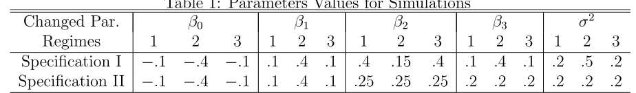
In specification I, the time series properties change greatly and the change points can be identified relatively easily. In specification II, it is challenging to capture the change points when the model structure is more stable. To make our simulation empirically realistic, we select parameter values of the HAR model which are close to those reported in Andersen, Bollerslev and Diebold (2007). They are listed in Table 1. For example, in specification I, if there is 1 break, β0 changes from −0.1 to−0.4. If there are two breaks,
it changes from −0.1 to −0.4 and finally to−0.1.
For each model, we generate T = 1000 observations. The true models we consider include cases of no change point, 1 and 2 change points. When there is 1 change point, the position of this change point follows a uniform distribution U(0.25×T,0.75×T). When there are 2 change points, the first one followsU(0.2×T,0.4×T) and the second follows U(0.6×T,0.8×T). This setting allows us to account for the randomness of the change points as well as ensuring sufficient observations in each regime to conduct an estimation.
In the following, the model specifications assumed are known but the number of struc-tural breaks and model parameters are unknown. For each draw from the DGP, we estimate the change-point model assuming 0,1,2,and 3 structural breaks. We rank the evidence for the number of break points according to the largest ML. The best change point specification has the largest ML, while the second best has the next largest, etc. We draw a new sample of data from the DGP and repeat this until 100 repetitions are completed. Then we report the frequency of repetitions in which each specification isbest
according to ML.
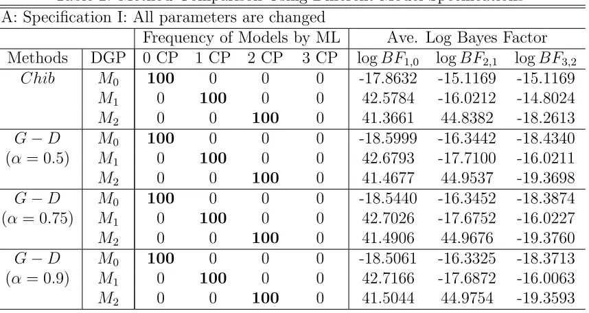
The comparison results of the two methods are summarized in table (2). Panel A is for specification I and Panel B for specification II. The second column indicates the underlying DGP. The 3−6 columns report the frequency over 100 repetitions in which each model isbest according to ML. For convenience, bold entries in these cells should be
100 if classification is perfect. For example, the first entry tells when underlying DGP is stable (M0). Out of 100 repetitions, 100 are correctly identified as no change point while
0 are identified incorrectly as 1, 2, or 3 change points according to the Chib method. The next entry in the table repeats this for a DGP with 1 change point (M1). Here, 100
times the 1 change point is correctly identified. For this ”easy” specification, the model ranking results from the Chib and GD methods are identical. The frequencies in their corresponding cells are all 100.
The last three columns report the average log BF over the 100 repetitions, with logBFi,j denoting the log BF of the model with i change points to the model with j
change points. Those numbers are fairly close across the two methods. For example, when underlying DGP is stable (M0), the log BF of the model with 1 change point to
the stable model logBF1,0 is −17.8632 by the Chib method and−18.5999,−18.5440 and
−18.5061 by the GD method witha= 0.5,0.75 and 0.9 respectively. This means although the GD and Chib methods calculate different marginal likelihoods, they provide almost identical evidence for the relative strengthen between two models.
Panel B contains the results from the more challenging specification II, where only the first two parameters are allowed to change. The results are very similar to the first case. The frequencies with which the two methods can correctly identify the underlying
DGP are very close: When underlying DGP is stable, 99 out of 100 repetitions are correct by the Chib method, and 100,98,98 by the GD method. When underlying DGP have 1 or 2 changes points, these numbers are 90 or 95 by the Chib method, and 94,93,93 or 97,96,96 by the GD method respectively. Furthermore, their corresponding log BF are roughly the same. Therefore, model comparison and selection using the two methods reports similar results.
In summary, when calculating ML, the Chib and GD methods with differenceα prefer the same candidate model. As a result, it is safe to choose GD method under usual conditions (the parameters are not more than 20).
References
[1] Andersen, T. G., T. Bollerslev and F. X. Diebold, 2007. Roughing It Up: Including Jump Components in the Measurement, Modeling and Forecasting of Return Volatil-ity. Review of Economics and Statistics, 89, 701-720.
[2] Chib, S., 1995. Marginal likelihood from the Gibbs output. Journal of the American Statistical Association, 90(432), 1313–1321.
[3] Chib, S., 1998. Estimation and comparison of multiple change point models. Journal of Econometrics, 86, 221-241.
[4] Corsi, F., 2009. A simple long memory model of realized volatility. Journal of Financial Econometrics, 7(2), 174-196.
[5] Gelfand, A. E. and Dey, D. K., 1994. Bayesian model choice: asymptotics and exact calculations. Journal of the Royal Statistical Society, B 56, 501-514.
[6] Geweke J., 1999. Using Simulation Methods for Bayesian Econometric Models: Infer-ence, Development, and Communication. Econometric Reviews, 18, 1-126.
[7] Kass, R. E. and A. E. Raftery, 1995. Bayes factors and model uncertainty. Journal of the American Statistical Association, 90, 773-795.
[8] Liu, C. and J. M. Maheu, 2008. Are there Structural Breaks in Realized Volatility? Journal of Financial Econometrics, 6(3), 326-360, Summer, 2008.
Table 1: Parameters Values for Simulations
Changed Par. β0 β1 β2 β3 σ2
Regimes 1 2 3 1 2 3 1 2 3 1 2 3 1 2 3 Specification I −.1 −.4 −.1 .1 .4 .1 .4 .15 .4 .1 .4 .1 .2 .5 .2 Specification II −.1 −.4 −.1 .1 .4 .1 .25 .25 .25 .2 .2 .2 .2 .2 .2
This table lists the hypothetic parameter values for our Monte Carlo simulation. The first column is the changed parameters. The second column lists the index of the regimes. The first row is the Specification index.
Table 2: Method Comparison Using Different Model Specifications A: Specification I: All parameters are changed
Frequency of Models by ML Ave. Log Bayes Factor Methods DGP 0 CP 1 CP 2 CP 3 CP logBF1,0 logBF2,1 logBF3,2
Chib M0 100 0 0 0 -17.8632 -15.1169 -15.1169
M1 0 100 0 0 42.5784 -16.0212 -14.8024
M2 0 0 100 0 41.3661 44.8382 -18.2613
G−D M0 100 0 0 0 -18.5999 -16.3442 -18.4340
(α = 0.5) M1 0 100 0 0 42.6793 -17.7100 -16.0211
M2 0 0 100 0 41.4677 44.9537 -19.3698
G−D M0 100 0 0 0 -18.5440 -16.3452 -18.3874
(α= 0.75) M1 0 100 0 0 42.7026 -17.6752 -16.0227
M2 0 0 100 0 41.4906 44.9676 -19.3760
G−D M0 100 0 0 0 -18.5061 -16.3325 -18.3713
(α = 0.9) M1 0 100 0 0 42.7166 -17.6872 -16.0063
M2 0 0 100 0 41.5044 44.9754 -19.3593
B: Specification II: Only first two parameters are changed
Frequency of Models by ML Ave. Log Bayes Factor Methods DGP 0 CP 1 CP 2 CP 3 CP logBF1,0 logBF2,1 logBF3,2
Chib M0 99 1 0 0 -6.1262 -5.1291 -5.3248
M1 0 90 8 2 18.4132 -1.1588 -2.2764
M2 0 1 95 4 11.2407 17.3668 -1.7567
G−D M0 100 0 0 0 -6.4047 -5.4062 -5.9070
(α = 0.5) M1 0 94 6 0 18.5095 -1.5342 -2.7379
M2 0 0 97 3 9.9774 18.8452 -2.4243
G−D M0 98 2 0 0 -6.3441 -5.3698 -5.8625
(α= 0.75) M1 0 93 7 0 18.5339 -1.5018 -2.6975
M2 0 0 96 4 9.9590 18.9105 -2.4013
G−D M0 98 2 0 0 -6.3037 -5.3470 -5.8571
(α = 0.9) M1 0 93 7 0 18.5480 -1.4781 -2.6761
M2 0 0 96 4 9.9541 18.9412 -2.3863
This table reports the comparison results of calculating ML using GD method and Chib method for two model specifications. The second column indicates the underlying DGP. The 3-6 columns display the number of times in the 100 repetitions when that specification had the largest ML. The last three columns report the average log BF between two models.