Chaos Synchronization of Uncertain Lorenz System via Single State Variable Feedback

(1)

http://dx.doi.org/10.4236/am.2013.411A2002

Chaos Synchronization of Uncertain Lorenz System via

Single State Variable Feedback

Fengxiang Chen1,2*, Tong Zhang1,2 1

School of Automotive Studies, Tongji University, Shanghai, China

2

Clean Energy Automotive Engineering Center, Tongji University, Shanghai, China Email: *[email protected]

Received May 6, 2013; revised June 6, 2013; accepted June 13, 2013

Copyright © 2013 Fengxiang Chen, Tong Zhang. This is an open access article distributed under the Creative Commons Attribution License, which permits unrestricted use, distribution, and reproduction in any medium, provided the original work is properly cited.

ABSTRACT

This paper treats the problem of chaos synchronization for uncertain Lorenz system via single state variable information of the master system. By the Lyapunov stability theory and adaptive technique, the derived controller is featured as follows: 1) only single state variable information of the master system is needed; 2) chaos synchronization can also be achieved even if the perturbation occurs in some parameters of the master chaotic system. Finally, the effectiveness of the proposed controllers is also illustrated by the simulations as well as rigorous mathematical proofs.

Keywords: Uncertain Lorenz System; Single State Variable; Chaos Synchronization

1. Introduction

Chaos control and synchronization have been intensively investigated during last decade [1-3] and still have at- tracted increasing attention in recent years. Chaos synchronization has many potential applications in secure communication [1], laser physics, chemical reactor proc- ess [2], biomedicine and so on. Up to now, numerous methods have been proposed to cope with the chaos synchronization, such as backstepping design method [3], adaptive design method [4], impulsive control method [5], sliding mode control method [6,7], and other control methods [8-10]. But most of the proposed methods abovementioned need more single state variable information of the master system. However, for instance, the more state variables transmitted to the slave system means the more bandwidth and energy consumption in secure communication system as well as security reduc- tion. Additionally, controller based on single state variable is simple, efficient and easy to be implemented in practical applications [11]. For example, in a real engineering case, some state variables may be difficult or even cannot be detected.

Recently, scholars begin to have attention on the problem of chaos synchronization via single state variable controller (hereafter refereed to as “SSVC”) with the motivation of the above facts. Jiang Zhang [12] gives a

schematic method to design the synchronization controller for a class of chaos system based on backstepping design, and several elegant results derived. However, the controllers conceived by several high-degree complex polynomials. M. T. Yassen [11] provided linear SSVC to Lu chaotic system, but the gain of the controller is difficult to be determined due to the fact that it contains the information of the upper bound of the system trajectory. In order to overcome the deficiency, he modified the SSVC based on adaptive technique. Junan Lu [13] gave out an adaptive SSVC for an unified chaotic system (uni- fication of Lorenz, Chen and Lu chaotic system). Feng- xiang Chen [14] proposes a linear SSVC for Lu system via theory of cascade-connection system. However, lit- eratures [11-14] did not take the parameters uncertainty into account, and the synchronization failed when some uncertainty occurs. On the other hand, for an electrical or electronic system, parameter uncertainty is inevitably suffered due to the variation of temperature, humidity, voltage, or interference of electric and magnetic fields. Thus, in this paper, we will provide robust SSVC for uncertain Lorenz chaotic system based on Lyapunov stability theory, and its effectness is validated by both rigorous theoretical analysis and simulations.

The rest of this paper is organized as follows. In the next section, the problem statement on the scheme of master-slave chaos synchronization for uncertain Lorenz system via single state variable information is presented.

(2)

In Section 3, three controllers are provided to the Lorenz system without/with parameters perturbation. In Section 4, numerical simulations are provided to illustrate the effectiveness of the proposed controllers. Finally, some conclusion remarks are included in Section 5.

2. Problem Formulation

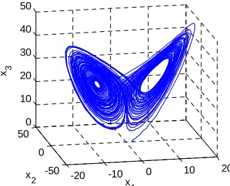
The Lorenz system is a system of ordinary differential equations (the Lorenz equations defined by (1)) first studied by Edward Lorenz [15]. It is notable for having chaotic solutions for certain parameter values and initial conditions. In particular, the Lorenz attractor is a set of chaotic solutions of the Lorenz system. Consider the Lo- renz system:





1 2 1

2 1 2 1 3 1 2 3

x x x

3

x rx x x x

x x x bx



      

  

(1)

where , ,r b are system parameters, x x x1, 2, 3 are

state variables, the system generates the chaotic behavior (see Figure 1) when  10,r28,b8 3. Hereafter in this paper, we refer to the system (1) as master system and assume that x1 is the only available state variable.

The related slave system with control inputs are writ- ten as





1 0 2 1 1

2 0 1 2 1 3 2

3 1 2 0 3 3

ˆ ˆ ˆ

ˆ ˆ ˆ ˆ ˆ

ˆ ˆ ˆ ˆ

x x x u

x r x x x x u

x x x b x u



         



 

(2)

where 0, ,r b0 0 are system nominal parameters and 1 2

ˆ ˆ, ,ˆ₃

x x u D

x 4

: R R

are state variables, i.e.

i , and they will be work out

later.



1,ˆ ˆ1, 2,ˆ3



,

i i

u u x x x x

, 3 ,i1, 2

tion

Our target is to find out the func u i_i, 1, 2, 3 such that the trajectory of the slave system (2) is going to asymptotically approach the master system (1) and finally implement chaos synchronization in the sense that

-20 -10 0 10 20

-50 0 50

0 10 20 30 40 50

x

1

x

2

[image:2.595.89.254.565.699.2]

x 3

Figure 1. Lorenz chaos phenomenon at 10, r28, 8 3

b .

lim i 0, 1, 2, 3

te  i where .

ˆ

i i

e  x x_i

3. Controller Design

According to the parameter uncertainties, we can classify the synchronization system into 8 cases listed in Table 1.

If we introduce the set A B C, , defined as following:







, , , 0, ,0 0 0, 0, 0



A  r b r b   rr bb







, , , 0, ,0 0 0, 0, 0



B  r b r b   rr bb



 





2 2



0 0 0 0 0

, , , , , 0

C  r b r b rr  b b 

Obviously, it is an equivalent partition for the element from case 1 to case 8. i.e., Acase 1, Bcase 2,

3

i

. Consequently, in this section, we are only going to investigate the chaos synchronization under three different classifications defined by the set

8

case

C



i

, ,

A B C.

C1:



, , ,r b0, ,r b0 0



A

Theorem 1: The two Lorenz chaotic systems (1) and (2) can be synchronized under the control law as follows:

1

2 0 1 0 1 1 3 1 3

3 1 2 1 2

0

ˆ ˆ ˆ ˆ

ˆ ˆ ˆ

u

u r x r x x x x x

u x x x x

 

     

   

(3)

Proof: Subtracting Equation (1) from Equation (2), then the error dynamic system is obtained as





1 0 2 1 2 2 1 3 3 1 2 0 3

e e

e e x e

e x e b e

 e

      

  

(4)

Choosing the Lyapunov function as

2

2 2 1

2 3 0

1

2 2

2

e

V e





   

 e 

 

2

(5)

and taking the derivative along the trajectory of the system (4), it yields

2 2

1 1 2 2 1 2 3 1 2 3 0 3

2 2 2

1 2 1 2 0 3

2 2 2 2

2 2 0

V e e e e x e e x e e b e

e e e e b e

            



(6)

The proof is completed.

C2:



, , ,r b0, ,r b0 0



B

For this case, the system (1) can be equivalent to the perturbation system as

Table 1. Synchronization system classification based on parameter uncertainties.

Case 1 Case 2 Case 3 Case 4 Case 5 Case 6 Case 7 Case 8

0 0

0

r r

b b

   

0 0

0

r r

b b

   

0 0

0

r r

b b

   

0 0

0

r r

b b

   

0 0

0

r r

b b

   

0 0 0

r r

b b

   

0 0

0

r r

b b

   

0 0

0

r r

b b

[image:2.595.309.540.674.734.2]

(3)

1





1 0 2 1 2 0 1 2 1 3 3 1 2 0 3

x x x

x r x x x x

x x x b x



       

  



1

(7)

where . h0





1 0 2 1 1 1 1 2 2 1 3

3 1 2 0 3

e e e e

e e x e

e x e b e

 

    

  

 

  

where  1



  0



x2x



. e

(9) Since the trajectory of the master system (1) is

bounded due to the property of chaos system, 1 must

be bounded, i.e. M1 R , . .s t 1 M1 

    .

Theorem 2: The two Lorenz chaotic systems (1) and (2) can be synchronized under the control law as follows:



2

2 2 *

1

2 3

0 0

1 1

2 2

e

V e e

h  



 

 

     

  (10)





1 1 1 1 1

2 0 1 0 1 1 3 1 3 3 1 2 1 2

1 1

ˆ ˆ

ˆ ˆ ˆ ˆ

ˆ ˆ ˆ

ˆ

u x x x x

u r x r x x x x x

u x x x x

h x x



   



   



  



  



(8) _where*

is a constant and will be determined later. Taking the derivative along the trajectory of the system (4), it yields









* 1

2 2 2 1 1

1 1 2 2 1 2 3 1 2 3 0 3

0 0 0

* 1 1 1 1

2 2 2

1 2 0 3

0 0 0

*

1 1 1

2 2 2

1 2 0 3

0 0

2 2 2 2

1 3

2

2 2

1 3

2

2 2

e e

V e e e e x e e x e e b e

h

e

e e

e e b e

e e

e e b e

   

  

  

  



 

 

         

 

      



     

 

(11)

If we select   * 1 , then V0. Theorem 3: The two Lorenz chaotic systems (1) and

(2) can be synchronized under the control law as follows:

Comment 1: Since the controller input component

1 1

e e (see Equation (8)) is not continuous at e10, it

leads to chattering in the viewpoint of engineering appli-cation. In order to overcome this defect, a continuous function 2 arctan

 

ke1  is adopted to substitute the

discontinuity function e1 e1 based on the conception

of variable structure controller design theory, and thus the chattering will be eliminated.





1 0 1 1

2 0 1 0 1 1 3 1 3 3 1 2 1 2

ˆ

ˆ ˆ ˆ ˆ

ˆ ˆ ˆ

u M x x

u r x r x x x x x u x x x x



 

 

    

   

(14)

where 1





2 1 2

1 1 2 0 2 2 3 1 2

3

M  M  M M ,













1 2 1 0

0,1 2 , 0, 3 2 , 0, 2b .

     

C3:



, , ,r b0, ,r b0 0



C

In this case, the system (1) can be equivalent to the

perturbation system as

_

_

1 0 2 1 1 2 2 1 3 2 3 1 2 0 3 3

e e e M

e e x e

e x e b e



             

  

1

e

(15)





1 0 2 1 1 2 0 1 2 1 3 2 3 1 2 0 3 3

x x x

x r x x x x

x x x b x



            

  

(12)

where 2

2 2 1

2 3 0

1

2 2

2

e

V e





 _  

 e 



 (16)















1 0 2

2 0 1

2 0 3

1

x x

r r x

b b x

 

      

  

(13) and taking the derivative along the trajectory of the system (4), it yields





2 2 2

1 1 2 2 1 2 3 1 2 3 0 3 1 1 0 2 2 3 3

2 2 2 2

V e e e e x e e x e e b e M

e  e e

             



(17) Since the trajectory of the master system (1) is

bounded, i must be bounded, i.e. Mi R , 

 

. . _i _i

s t  M . Additionally, if   0, rr0, bb0

then  1 0,  2 0, and  3 0 respectively.

Note that , for any ,

thus

2 1

(4)





























2 2 2

1 2 1 2 0 3 2

1 2 1 2 2 1

1 1 0 1 1 2 2 2 2 3 3 3 3

2 2 2

1 1 2 2 0 3 3

2

1 1 2 1 2

1 1 0 2 2 3 3

2 2

2

1 2 3 2 2

2

V e e e e b e M

e e

e e b e M

2 2

e

      

  

   

 

  

     

        

       

     





(18) Note that 1



0,1 2 ,



2



0, 3 2 ,



1



0,b0



, and









2

1 1 2

1 1 2 0 2 2 3

M      12

3 

(19)

then V0. The proof is completed.

Comment 2: Although the component of input 1

will increase to infinity as 1 1

u ˆ

x x, so the law is only a conceptional controller and can not be implemented in real application. But this does not mean that the controller law is meaningless. In real implementation, we can modify the u1 as









0 1 1 1 1

1 2

0 1 1 1 1

ˆ ˆ

M x x x x r

u

M x x r x x r

 

  

  

 



 



2 3



(20)

With the modified controller, the synchronization error will not approach to zero, but in the vicinity of the

, the details see [16] and simulation 3. On the other hand, the errors of 2 3 is independent of

and , but decided by the following subsystem:



0, 0, 0

1

u

,

e e e1

2 2 1 3 3 1 2 0 3

e e x e

e x e b e

    

   



 (21)

which means that any effort on the 1 will not have any

beneficial to attenuate the fluctuation of . u

2, 3

e e

4. Numerical Simulation

In this section, three numerical simulations named as Simulation 1, Simulation 2 and Simulation 3 are carried out to illustrate the effectiveness of the proposed controller. For sake of simplification, we refer the controller defined by (3) to as nominal controller, the controller defined by (8) to as adaptive controller, and the controller defined by (14) to as robust controller in the following simulations.

Simulation 1:

In this subsection, we are going to validate the effectiveness of nominal controller designed under the condi-

tion . Thus, three parameters of

Lorenz master system and slave system are chosen iden- tically as



, , ,r b0, ,r b0 0 A

0 10,r r0 28,b b0 8 3

  

 

1 0 2, 2 0 0, 3 0

x  x  x



 

ˆ 0 1.1,ˆ 0 0.2,ˆ

x  x 

   

 

. Initial states of the master and slave system are taken as

and 0



x

 

0

1 2 3 , respectively, and they

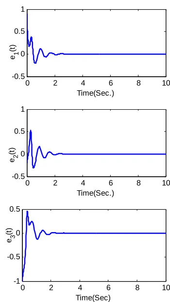
will be kept the same through out the following simulations. Taking the control input as the nominal controller, the simulation results are shown in Figure 2. As we can

1

0 2 4 6 8 10

-0.5 0 0.5 1

Time(Sec.) e 1

(t

)

0 2 4 6 8 10

-0.5 0 0.5 1

Time(Sec.) e 2

(t

)

0 2 4 6 8 10

-1 -0.5 0 0.5

Time(Sec) e3

(t

[image:4.595.333.508.81.392.2]

)

Figure 2. Synchronization errors with the nominal control- ler for Lorenz system without uncertainty.

see that the synchronization is achieved after about 3 seconds. Which means that the nominal controller is ef- fective for the synchronization system without uncertainty; however, this is not the case when the parameter perturbations are occurred and the results are shown in the subsequently Simulation 2 and Simulation 3.

Simulation 2:

In this subsection, we add the parameter 30% perturbations to  , i.e.,  13,. The adaptive controller defined by (8) is taken as









 

1 1

2 0 1 0 1 1 3 1 3 3 1 2 1 2

1 1

ˆ arctan 800

ˆ ˆ ˆ ˆ

ˆ ˆ ˆ

ˆ

100 , 0 5

u x

u r x r x x x x x

u x x x x

x x



 

  



   



 _ _

 

1

x

  



(22)

which has been modified according to the Comment 1. And the results are shown in Figure 3. We can see that the synchronization via nominal controller is failed due to the fluctuation of e t1

 

. Meanwhile, the synchroniza-

(5)

0 5 10 -4

-2 0 2 4

e1

(t

)

Time(Sec.)

0 5 10

-0.4 -0.2 0 0.2 0.4

e 2

(t

)

Time(Sec.)

0 5 10

-1 -0.5 0 0.5

e 3

(t

)

Time(Sec.)

0 5 10

5 10 15 20 25



(t

)

Time(Sec.) Adaptive Controller

Nominal Controller

Adaptive Controller Nominal Controller

[image:5.595.149.449.85.308.2]

Adaptive Controller Nominal Controller

Figure 3. Synchronization errors for uncertain Lorenz system via the adaptive controller and nominal controller, respec- tively.

r

achieved. On the other hand, the perturbation of parame-

0 2 4 6 8 10

-2 2

te  13 hardly has any impact on the convergence of

3

(23)

is independent of

   

2 , 3

e t e t due to the subsystem

2 2 1 3

e e x e

e x e b e

  

 



₃ _{1 2} ₀  and

proved that the sub ystem 3) is asymptotically stable

1

e .

(2

It can be easily to be s

(i.e. xˆ2x x2,ˆ3x3 as t) with any x1. For

example, choosing Lyapunov function as V e22e32,

then . W eans that the nver-

gence rate of ˆ2,ˆ3 2 2 0

V  e be32 0 hich m co

x x is independent of the p of

erturbation

 and e1. : Simulation 3

In this su secb tion, we are going to analysis the per- fo st controller designed under the condi- tio

rmance of robu

n



, , ,r b0, ,r b0 0



C. Here we consider the worst

case, i.e.   0,rr b0, b0. The parameters of the

master system are taken as  13 (+30% perturbation of the nominal value 10), r23.8 (15% perturbation of the nominal value 28), b3.2 (+20% perturbation of the nominal value 8/3). R ntroller and nominal controller are here both ado as to compare their performance on the chaos synchronization and the simulation results are shown in Figure 4. From Figure 4, we can see that the synchronization via nominal controller and robust controller are both failed due to the errors do not converge to zero but undulate in a bounded area. For robust controller,



obust pte

co d so



1

e t approaches to zero, but this is not the case for other error component e t2

 

and e t3

 

,

which has been interp ted by Comment 2. For nominal controller, all error components

re

 

1 t ,

e e t₂

 

and

0

Robust Controller Nominal Controller e1

(t

)

0 2 4 6 8 10

-5 0 5

e 2

(t

)

Robust Controller Nominal Controller

0 2 4 6 8 10

-10 -5 0

e3

(t

)

Time(Sec.)

Robust Controller Nominal Controller

Figure 4. Synchronization errors for uncertain Lorenz sys- tem via the robust controller and nominal controller, re- spectively.

 

3

e t varied in the vicinity of certain value, respectively. As mentioned in Comment 2, the error component e t2

 

and e t3

 

is independent of and , but decided

y (21). Wh

1

e th 2

1

u and

b ich means that bo e t

 

e t3

 

must

[image:5.595.327.521.350.615.2]

(6)

and orresponding numerical simulation result are shown in Figure 4.

5. Conclusion

the c

edback of single state variable from ing to parameter uncertain tion is defined to classify the parame-

r

more effectively b .

d I d National Nature Science

77].

Synchro- nization and Secure Communication,” Philosophical

Transactions of th o. 1911,

2010, pp.

379-The paper investigates the synchronization of uncertain Lorenz system via fe

the master system. Accord an equivalent parti

ties,

ter uncertain Lorenz system. Then three controllers (nominal controller, adaptive controller, and robust controller) are given out to achieve the chaos synchronization based on Lyapunov stability theory and adaptive technique. Finally, three numerical simulations are conducted to validate the effectiveness of the proposed controllers, and it finds that the adaptive controllers do really elimi- nate the disturbance caused by parameters perturbation but it is not the case for nominal controller. For robust controller, any effort to modify the controller u1 will

not have beneficial to attenuate the error component

 

2

e t and e t3

 

which is independent of e1 and u1,

but decided by (21). For the future investigation, we will use L2 gain theory and passivity theory to design a obust

synchronization controller to attenuate the disturbance ased on single state variable

6. Acknowledgements

This work is supported by National Special Fund for the Development of Major Research Equipment an nstru- ments [2012YQ150256], an

Foundation of China [611040

REFERENCES

[1] W. Kinzel, A. Englert and I. Kanter, “On Chaos

e Royal Society A, Vol. 368, N

389.

http://dx.doi.org/10.1098/rsta.2009.0230

[2] S. Rasoulian and M. Shahrokhi, “Control of a Chemical Reactor with Chaotic Dynamics,” Iranian Journal of Chemistry & Chemica

pp. 149-159.

l Engineering, Vol. 29, No. 4, 2010,

[3] X. Tan, J. Zhang and Y. Yang, “Synchronizing Chaotic Systems Using Backstepping Design,” Chaos, Solitons &

Fractals, Vol. 16, No. 1, 2003, pp. 37-45.

http://dx.doi.org/10.1016/S0960-0779(02)00153-4

[4] F. Sorrentino, G. Barlev, A. B. Cohen and E. Ott, “The Stability of Adaptive Synchronization of Chaotic Sys- tems,” Chaos, Vol. 20, No. 1, 2010, Article

http://dx.doi.org/10.1063/1.3279646

[5] M. Haeri and M. Dehghani, “Impulsive Synchronization of Different Hyperchaotic (Chaotic) Systems,” Chaos,

Solitons & Fractals, Vol. 38, No. 1, 2008, pp. 120-131.

http://dx.doi.org/10.1016/j.chaos.2006.10.051

[6] H.-T. Yau, “Design of Adaptive Sliding Mode Controlle for Chaos Synchronization with Uncertaintie

r

s,” Chaos,

Solitons & Fractals, Vol. 22, No. 2, 2004, pp. 341-347.

[7] C.-C. Wang and J.-P. Su, “A New Adaptive Variab Structure Control for Chaotic Synchronization an

le d Secure Communication,” Chaos, Solitons & Fractals, Vol. 20, No. 5, 2004, pp. 967-977.

[8] X. Yu and Y. Song, “Chaos Synchronization via ling Partial State of Chaotic Systems,” In

Control-

ternational

Journal Bifurcation and Chaos, Vol. 11, No. 6, 2001, pp.

1737-1741.

http://dx.doi.org/10.1142/S0218127401003024

[9] X.-F. Wang, Z.-Q. Wang and G.-R. Chen, “A N rion for Synchronization of Coupled Chaotic Oscillato

ew Crite- rs with Application to Chua’s Circuits,” International Jour-

nal Bifurcation and Chaos, Vol. 9, No. 6, 1999, pp. 1169-

1174. http://dx.doi.org/10.1142/S021812749900081X

[10] J. Cao, H. X. Li and D. W. C. Ho, “Synchronization Cri- teria of Lur’s Systems with Time-Delay Feedback Con-

stem,” Chaos Solitons and Fractals, Vol. trol,” Chaos, Solitons and Fractals, Vol. 23, No. 4, 2005, pp. 1285-1298.

[11] M. T. Yassen, “Feedback and Adaptive Synchronization of Chaotic Lu sy

25, No. 2, 2005, pp. 379-386.

[12] J. Zhang, C. G. Li, H. B. Zhang and J. B. Y Synchronization Using Single Variable Feedb

u, “Chaos ack Based on Backstepping Method,” Chaos Solitons and Fractals, Vol. 21, No. 5, 2004, pp. 1183-1193.

[13] J. A. Lu, X. Q. Wu, X. P. Han and J. H. Lü, “Adaptive Feedback Synchronization of a Unified Chaotic System,”

Physics Letters A, Vol. 329, 2004, pp. 327-333.

http://dx.doi.org/10.1016/j.physleta.2004.07.024

[14] F. X. Chen, C. S. Zhang, G. J. Ji, S. Zhai and

“Chua System Chaos Synchronization Using Single S. Zhou,

to Turbulence,” John

, 2007. Variable Feedback Based on Lasalle Invariance Princi- pal,” Proceedings of the 2010 IEEE International Con-

ference on Information and Automation, Harbin, 20-23

June 2010, pp. 301-304.

[15] P. Bergé, Y. Pomeau and C. Vidal, “Order within Chaos: Towards a Deterministic Approach

Wiley & Sons, New York, 1984.

[16] H. K. Khalil, “Nonlinear Systems,” Third Edition, Pub- lish House of Electronics Industry, Beijing