Load Balancing for Hex Cell Interconnection Network

http://dx.doi.org/10.4236/ijcns.2016.94009

Load Balancing for Hex-Cell Interconnection

Network

Saher Manaseer1_{, Ahmad Alamoush}1_{, Osama Rababah}2

1_{Department of Computer Science, King Abdullah II School for Information Technology, The University of}

Jordan, Amman, Jordan

2_{Department of Business Information Technology, King Abdullah II School for Information Technology, The} University of Jordan, Amman, Jordan

Received 4 March 2016; accepted 26 April 2016; published 29 April 2016

Copyright © 2016 by authors and Scientific Research Publishing Inc.

This work is licensed under the Creative Commons Attribution International License (CC BY). http://creativecommons.org/licenses/by/4.0/

Abstract

The hex-cell is one of the interconnection networks used for parallel systems. The main idea of the hex-cell is that there are hexagon cells that construct the network; each one of those cells has six nodes. The performance of the network is affected by many factors one of the factors as load balanc-ing. Until the moment of writing of this paper, there is no load balancing algorithm for this network. The proposed algorithm for dynamic load balancing on hex-cell is based on Tree Walking Algo-rithm (TWA) for load balancing on tree interconnection network and the ring all to all broadcast.

Keywords

Hex-Cell, Load Balancing, Tree Walking

1. Introduction

Hex-cell is newly proposed interconnection network in (2008) [1]. The researches that evaluate the performance of the hex-cell are not enough and it should get more attention because it has potentials for parallel systems. Since there is no load balancing algorithm on hex-cell topology (until the moment of writing of this paper), the aim of this paper is to propose a dynamic load balancing algorithm and evaluate it.

The proposed algorithm is based on Tree Walking Algorithm (TWA) for load balancing on tree interconnec-tion network and the ring all to all broadcast, using the SBHCR (Secinterconnec-tion Based Hex-Cell Routing Algorithm) addressing schema proposed in that divides the hex-cell into six sections [2].

proposed load balancing algorithm and example to illustrate the way the algorithm works. Section 4 is the simu-lation for the algorithm. Finally, Section 5 is the conclusion of the paper and the future work.

2. Related Works

2.1. Hex-Cell Network Topology

Hexogen units create hex-cell topology; each one of those cells has six nodes. The depth of the network is the number of levels around the innermost cell denoted by HC (d) where d is the depth. So the innermost cell has depth of one, the six cells around it form level two, then the next twelve cells make the level three and so on [1], As shown in Figure 1.

There are three addressing for the hex-cell topology. First addressing depend on the number of the line that the node stand on from top to down and the number of node in that line from left to right [1], which denoted by pair (X, Y) where X is the line number and Y is the node number in that line. So if the node in the third line and has position of ten then the node label is (3, 10). As shown in Figure 2.

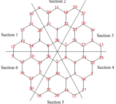
The second addressing of the hex-cell is by dividing the network into six sections label from one to six left to right (clockwise). Each node takes a label consist of three numbers (S, L, X) where S is the section number, L is the level number and X is the node number in that level while X is not bigger than ((2 × L) − 1) [2]. So if we have a node in section three, in level two and number in that level is three then the node label is (3, 2, 3). As shown in Figure 3.

The third addressing is by using the level of the node and the node number in that level. Which denoted by pair (X, Y) where X is the level number and Y is the node number while the Y is less than 6 × (2 × L − 1) where L is the node level [3]. So the node in the third level and has number of thirty then (3, 30) as shown in Figure 4.

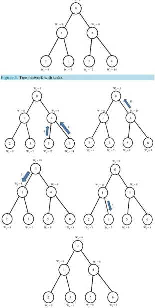
2.2. Tree Walking Algorithm (TWA)

The TWA uses global information collection to know the accumulative load at each subtree and the number of the nodes at each subtree. After that the root node calculates the average load and broadcast it. Then each node calculates the quota for subtree for which it is the root. Finally start the exchange of tasks between the nodes [4].

To explain how TWA works Figure 5 shows tree with seven nodes. Each node has number of tasks.

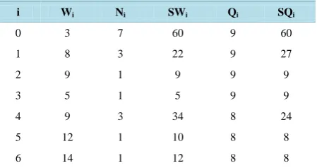
First after the global information collection, each node has number of tasks (Wi) and number of nodes in the subtree it rooted (Ni). Then each node calculate the total number of tasks in the subtree (SWi). The root node (N0) calculates the average load and the remaining task (R) that cannot be evenly divided on nodes. Then broadcast average load and R to all the nodes. Next each node calculates the quota for itself (Qi) and the subtree it rooted (SQi). Table 1 shows the values for each node.

The flow of steps is presented in Figure 6.

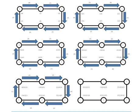
2.3. Ring All to All Broadcast

In all to all broadcast what needed is that each node sends the same message to all other nodes. That kind of

Figure 2. Hex-cell addressing by line number [1].

Figure 3. Hex-cell addressing by section [2].

Figure 5. Tree network with tasks.

Table 1. Calculate values for each node.

i Wi Ni SWi Qi SQi

0 3 7 60 9 60

1 8 3 22 9 27

2 9 1 9 9 9

3 5 1 5 9 9

4 9 3 34 8 24

5 12 1 10 8 8

6 14 1 12 8 8

broadcast on ring topology need (n − 1) communication steps where n is the number of nodes.

To explain how all to all broadcast on ring topology works Figure 7 shows ring topology consist of six nodes. Since the number of nodes equal six then the number of communication steps needed for all to all broadcast is five (6 − 1 = 5). First step each node sends its message to the next node clockwise. Then after that in the follow-ing four steps each node sends the recent message received from the previous node [5] as shown in Figure 8.

3. LBHC Proposed Algorithm

The proposed load balancing algorithm depends on the TWA on tree and all to all broadcast on ring. The hex- cell interconnection network in [2] is divided into six sections. We will use each section as tree topology and the root node for each tree construct ring topology of six nodes, as shown in Figure 9.

3.1. LBHC Algorithm

Phase one: Global information Collection

For each child in the node children {

Receive global information from the child} If node has parent {

Send global information to the parent } Else {

Calculate average load (accumulate task / accumulate nodes) Calculate remaining load (accumulate task Mod accumulate nodes)}

Phase Two: All to All ring broadcast

If node is root node { For six loops {

Send node global information to the next root node Receive global information from the previous root node} // Evaluate tasks load

If (maxAverage − minAverage > 5){

Calculate new global average load tasks (total task load / 6) Calculate new global remaining tasks (total task load Mod 6) Calculate new average load tasks (global average load / tree nodes) Calculate new remaining tasks (global average load Mod tree nodes)} }

Phase Three: Broadcast the Average Load

If node has parent {

Receive global information from the parent} For each child in the node children {

Send global information for the child} Calculate the Quota for each subtree

Phase Four: TWA balancing // Receiving

If ((Actual accumulated tasks < Quota){ Receive tasks from the parent}} For each child in the node children {

If ((Actual accumulated tasks for the child > Quota){ Receive tasks from the child}}

// Sending

For each child in the node children {

If ((Actual accumulated tasks for the child < Quota){ Send tasks to the child}}

If node has parent {

If ((Actual accumulated tasks > Quota){ Send tasks to the parent}}

Phase Five: Ring Balancing

If node is root node { For two loops {

Send (extra tasks or Zero tasks) to the next root node Receive extra tasks from the previous root node}}

Phase Six: Final Balancing

If node has parent {

If ((Actual accumulated tasks < Quota){ Receive tasks from the parent}} For each child in the node children {

If ((Actual accumulated tasks for the child < Quota){ Send tasks to the child}}

3.2. LBHC Phases

3.2.1. Phase One: Global Information Collection

Local information collection in each tree topology separately, as in TWA.

3.2.2. Phase Two: All to All Ring Broadcast

Each root node in the ring topology broadcast total task and average load to all other root nodes in the ring. Evaluate average load between the trees to check if it’s efficient to do global load balancing.

If it’s efficient to do global balancing then new global average load tasks and remaining tasks for each tree calculated as following:

1) The new average calculated by all root nodes:

a) Calculate new global average load tasks (accumulate task/6). b) Calculate new global remaining tasks (accumulate task Mod 6). 2) Tree task quota calculated by all root nodes:

a) Tree task quota = global average load + 1 IF section ≤ global remaining tasks. b) Tree task quota = global average load IF section > global remaining tasks. 3) Average load tasks and remaining tasks for each node calculated:

a) Calculate new average load tasks (global average load/tree nodes). b) Calculate new remaining tasks (global average load Mod tree nodes).

If is not efficient to do global balancing leave the average load and remaining task for each tree as it is.

Figure 8. All to all broadcast on ring topology.

3.2.3. Phase Three: Broadcast the Average Load

Broadcast the average load tasks and the remaining tasks for each node in the tree section. Each node calculates its quota:

1) Node quota = average load tasks + 1 IF node order < remaining tasks. 2) Node quota = average load tasks IF node order ≥ remaining tasks. For the each subtree quota:

Subtree quota = (Average load tasks × Number of nodes in the rooted subtree) + Remaining tasks for the rooted subtree.

3.2.4. Phase Four: TWA Balancing Trees with different load tasks do:

1) Trees with extra tasks apply TWA so that the extra task goes to the root node. 2) Trees with exact quota just apply TWA.

3) Trees with fewer tasks than its quota do TWA to complete its node from bottom to top with the right num-ber of tasks (the node quota).

3.2.5. Phase Five: Ring Balancing

If the root node has extra tasks then sends the extra tasks to the next root else it sends Zero tasks to the next root node.

3.2.6. Phase Six: Final Balancing

Apply TWA again to balance the received tasks.

3.3. LBHC Example

Here is an example on the proposed LBHC algorithm. Figure 10 shows hex-cell network and each node has number of tasks.

3.3.1. Phase One: Global Information Collection

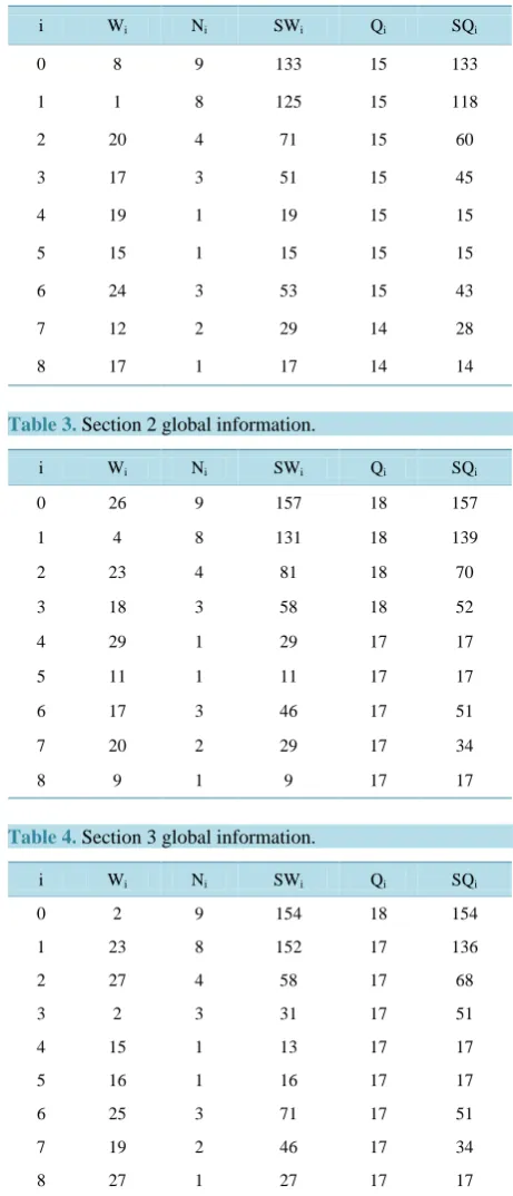
Each tree does the global information collection and compute total number of tasks and number of nodes in each subtree. The following six tables (Tables 2-7) show that information.

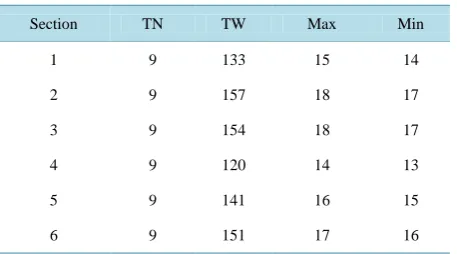
3.3.2. Phase Two: All to All Ring Broadcast

Each root node sends the maximum average and minimum average. Then evaluate the task number and it is effi-cient to do global balancing since maximum quota is 18 and the minimum is 13. (Since we have chosen 5 tasks different between the highest average tasks load and lowest average tasks load to check the efficiency to do

Table 2. Section 1 global information. SQi Qi SWi Ni Wi i 133 15 133 9 8 0 118 15 125 8 1 1 60 15 71 4 20 2 45 15 51 3 17 3 15 15 19 1 19 4 15 15 15 1 15 5 43 15 53 3 24 6 28 14 29 2 12 7 14 14 17 1 17 8

Table 3. Section 2 global information.

SQi Qi SWi Ni Wi i 157 18 157 9 26 0 139 18 131 8 4 1 70 18 81 4 23 2 52 18 58 3 18 3 17 17 29 1 29 4 17 17 11 1 11 5 51 17 46 3 17 6 34 17 29 2 20 7 17 17 9 1 9 8

Table 4. Section 3 global information.

SQi Qi SWi Ni Wi i 154 18 154 9 2 0 136 17 152 8 23 1 68 17 58 4 27 2 51 17 31 3 2 3 17 17 13 1 15 4 17 17 16 1 16 5 51 17 71 3 25 6 34 17 46 2 19 7 17 17 27 1 27 8

global balancing between the sections trees). So calculate the new tree quota. Table 8 shows the information broadcast to all root nodes.

So average load = total task/6. Average load = 856/6.

Average load = 142 and TR = 4.

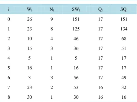
Table 5. Section 4 global information. SQi Qi SWi Ni Wi i 120 14 120 9 8 0 106 14 112 8 8 1 53 14 40 4 7 2 39 13 33 3 14 3 13 13 17 1 17 4 13 13 2 1 2 5 39 13 64 3 14 6 26 13 50 2 22 7 13 13 28 1 28 8

Table 6. Section 5 global information.

SQi Qi SWi Ni Wi i 141 16 141 9 2 0 125 16 139 8 30 1 64 16 76 4 18 2 48 16 58 3 22 3 16 16 16 1 16 4 16 16 20 1 20 5 45 15 33 3 7 6 30 15 26 2 14 7 15 15 12 1 14 8

Table 7. Section 6 global information.

SQi Qi SWi Ni Wi i 151 17 151 9 26 0 134 17 125 8 23 1 68 17 46 4 10 2 51 17 36 3 15 3 17 17 5 1 5 4 17 17 16 1 16 5 49 17 56 3 3 6 32 16 53 2 23 7 16 16 30 1 30 8

Tree quota = tree average load IF section > TR.

Then the quota for trees in Sections 1 to 4 is 143 while for trees in Sections 5 and 6 is 142. Each tree calculates the quota for each node and subtrees using the new average load. As following: The average load = 143/9 = 15 and the remaining (R) = 8.

Table 8. Section 5 global information.

Min Max

TW TN

Section

14 15

133 9

1

17 18

157 9

2

17 18

154 9

3

13 14

120 9

4

15 16

141 9

5

16 17

151 9

6

3.3.3. Phase Three: Broadcast the Average Load

Broadcast the new average load tasks and remaining to the nodes in the tree sections and calculate the new quo-ta.

Qi = (The average load + 1) IF i < R. Qi = (The average load) IF i ≥ R.

Tables 9-14 show the new average load for each node and subtrees.

3.3.4. Phase Four: TWA Balancing

Trees 2, 3 and 6 have extra tasks so we apply TWA on them. As an example we take tree Section 2. Figure 11 shows the section two trees with the tasks load it has.

Now the exchanging of tasks between the nodes is done as the following:

Each node i waits to receive tasks from its parent if (SWi < Qi) or from its children j if (SWj > Qj) else the node i send tasks to its parent if (SWi > Qi) or to its children j if (SWj < Qj).

Seven communication steps needed to perform the balancing: 1) Send 13 tasks from node 4 to node 3.

2) Send 10 tasks from node 3 to node 2. 3) Send 5 tasks from node 3 to node 5. Send 17 tasks from node 2 to node 1. 4) Send 4 tasks from node 1 to node 0. 5) Send 1 tasks from node 1 to node 6. 6) Send 2 tasks from node 6 to node 7. 7) Send 6 tasks from node 7 to node 8. As shown in Figure 12.

Trees 1, 4 and 5 have fewer tasks than its quota so we apply TWA to complete its node from bottom to top with the right number of tasks (the node quota) and wait for more tasks. As an example we take tree Section 4. Figure 13 shows the tree Section 4 that has fewer tasks than its quota.

Now the exchanging of tasks between the nodes is done as the following:

Each node i waits to receive tasks from its parent if (SWi < Qi) or from its children j if (SWj > Qj) else the node i send tasks to its parent if (SWi > Qi) or to its children j if (SWj < Qj).

Six communication steps needed to perform the partial balancing: 1) Send 8 tasks from node 0 to node 1.

Send 1 tasks from node 4 to node 3. Send 13 tasks from node 8 to node 7. 2) Send 19 tasks from node 7 to node 6. 3) Send 17 tasks from node 6 to node 1. 4) Send 24 tasks from node 1 to node 2. 5) Send 15 tasks from node 2 to node 3. 6) Send 14 tasks from node 3 to node 5. As shown in Figure 14.

Table 9. Tree 1 average load. SQi Qi SWi Ni Wi i 143 16 133 9 8 0 127 16 125 8 1 1 64 16 71 4 20 2 48 16 51 3 17 3 16 16 19 1 19 4 16 16 15 1 15 5 47 16 53 3 24 6 31 16 29 2 12 7 15 15 17 1 17 8

Table 10. Tree 2 average load.

SQi Qi SWi Ni Wi i 143 16 157 9 26 0 127 16 131 8 4 1 64 16 81 4 23 2 48 16 58 3 18 3 16 16 29 1 29 4 16 16 11 1 11 5 47 16 46 3 17 6 31 16 29 2 20 7 15 15 9 1 9 8

Table 11. Tree 3 average load.

SQi Qi SWi Ni Wi i 143 16 154 9 2 0 127 16 152 8 23 1 64 16 58 4 27 2 48 16 31 3 2 3 16 16 13 1 13 4 16 16 16 1 16 5 47 16 71 3 25 6 31 16 46 2 19 7 15 15 27 1 27 8

3.3.5. Phase Five: Ring Balancing

Here, the root nodes start to send extra tasks among between them (Clockwise) starting from root node in tree Section 1.

1) Root node in tree Section 1 will send 0 tasks since it waits for tasks.

2) Root node in tree Section 2 will not receive any tasks and it will send the extra tasks (14 tasks) to the root node in tree Section 3.

Table 12. Tree 4 average load. SQi Qi SWi Ni Wi i 143 16 120 9 8 0 127 16 112 8 8 1 64 16 40 4 7 2 48 16 33 3 14 3 16 16 17 1 17 4 16 16 2 1 2 5 47 16 64 3 14 6 31 16 50 2 22 7 15 15 28 1 28 8

Table 13. Tree 5 average load.

SQi Qi SWi Ni Wi i 142 16 141 9 2 0 126 16 139 8 30 1 64 16 76 4 18 2 48 16 58 3 22 3 16 16 16 1 16 4 16 16 20 1 20 5 46 16 33 3 7 6 30 15 26 2 14 7 15 15 12 1 12 8

Table 14. Tree 6 average load.

SQi Qi SWi Ni Wi i 142 16 151 9 26 0 126 16 125 8 23 1 64 16 46 4 10 2 48 16 36 3 15 3 16 16 5 1 5 4 16 16 16 1 16 5 46 16 56 3 3 6 30 15 53 2 23 7 15 15 30 1 30 8

the received tasks (total extra tasks 25) and send it to root node in tree Section 4.

4) Root node in tree Section 4 will receive 25 tasks, while it has fewer tasks load than it quota then it will take the appropriate number of task (23 tasks) and send the rest (2 tasks) to the root node in tree Section 5.

5) Root node in tree Section 5 will receive 2 tasks, while it has fewer tasks load than it quota then it will take the appropriate number of task (1 task) and send the rest (1 tasks) to the root node in tree Section 6.

Figure 11. Tree Section 2 with tasks load.

Figure 13. Tree Section 4 with fewer tasks then it quota.

Figure 15. Hex-cell network partial balanced.

7) Root node in tree section 1 will receive 10 task, and its quota is completed now. As shown in Figure 16.

3.3.6. Phase Six: Final Balancing

After the root node in tree section 4 received the tasks to complete its quota as shown in Figure 17. The tree will apply TWA again to balance the received tasks.

One communication step needed to perform the balancing: 1) Send 7 tasks from node 0 to node 1.

As shown in Figure 18.

Finally the hex-cell network tasks load is balanced as shown in Figure 19.

4. Simulation

The simulation is done using JAVA programming language version (1.8.0_51) 64-bit, using multi-threading to simulate each node. The hardware specification for our simulation are:

1) Processor: Intel(R) Core(TM) i5-2450 M CPU @ 2.50 GHz. 2) RAM: 6.00 GB.

3) System type: Windows 7/64-bit.

As for the simulation we have chosen 5 different tasks between the highest average tasks load and lowest av-erage tasks load to check the efficiency to do global balancing between the sections trees.

The major factor to evaluate load balancing algorithm is the accuracy. After the simulation with different le-vels and different inputs for the load tasks for each node, LBHC proved to be effective. In all runs, the differ-ence between the highest task load and the lowest task load is one. (Unless it is not efficient to do global ba-lancing where the difference will be the factor we choose and that is 5).

The execution time for any algorithm is one of the important factors to evaluate the performance. So Figure 20 shows the average execution time for LBHC in various levels, from level one (hex-cell has 6 nodes) to level ten (hex-cell with 600 nodes).

Another factor we have studied is number of messages in the network while applying the LBHC algorithm. Figure 21 shows the average number of messages in various levels from level one (hex-cell has 6 nodes) to lev-el ten (hex-clev-ell with 600 nodes).

5. Conclusion and Future Work

Figure 16. Root nodes from the sections sending tasks.

Figure 17. Partial balanced tree Section 4 received more tasks.

Figure 18. Tree section 4 apply TWA again to balance the received tasks.

Figure 19. Hex-cell network tasks load balanced.

Figure 20. Average execution time in nanosecond for different levels.

work, the next step is to propose another load balancing algorithm and compare it with the proposed one. After that, we could do more research on other aspects of the hex-cell interconnection network to evaluate its perfor-mance.

References

[1] Sharieh, A., Qatawneh, M., Almobaideen, W. and Sleit, A. (2008) Hex-Cell: Modeling, Topological Properties and Routing Algorithm. European Journal of Scientific Research, 22, 457-468.

[2] Qatawneh, M., Alamoush, A. and Alqatawna, J. (2015) Section Based Hex-Cell Routing Algorithm (SBHCR). Inter-national Journal of Computer Networks and Communications, 7, 167-177.

[3] Mohammad, Q. and Khattab, H. (2015) New Routing Algorithm for Hex-Cell Network. International Journal of Fu-ture Generation Communication and Networking, 8, 295-306.http://dx.doi.org/10.14257/ijfgcn.2015.8.2.24

[4] Shu, W. and Wu, M.-Y. (1995) An Incremental Parallel Scheduling Approach for Solving Dynamic and Irregular Problems. Proceedings of the 24th International Conference on Parallel Processing, Oconomowoc, 4 October 1995, 143-150.