Munich Personal RePEc Archive
Long-run identifying restrictions on
VARs within the AS-AD framework
Pentecôte, J.-S.
CREM (UMR CNRS 6211), University of Rennes 1
31 October 2010
Online at
https://mpra.ub.uni-muenchen.de/34660/
Long-run identifying restrictions on VARs within the AS-AD framework
Jean-Sébastien Pentecôte, CREM–UMR CNRS 6211
This version, October 2010
Abstract:
Bayoumi and Eichengreen’s (BE, 1994) article has been very influent in the empirics of the
core-periphery view of fixed exchange rate agreements. They rely on the basic AS-AD
macroeconomic model in order to identify supply and demand shocks through long-run
restrictions in vector autoregressions. Doing this should enable one to assess the size of such
disturbances and the asymmetry between countries. While reference is usually made to
Blanchard and Quah (BQ, 1989), it is shown here how this factorization has been modified by
BE and how the two resulting decomposition schemes can be linked. Contrary to BE’s
premise, relaxing the assumption of shocks of equal size is not just a matter of scale. The
empirical properties of the exchange regime are modified, especially as regards the
correlation of shocks. Given the VAR setting used in the related studies, it is also established
that zero-constraints on either instantaneous or long-run impulse responses provide
identical results. An empirical assessment of the euro currency area over 1996-2008
illustrate these points. The recorded evidence suggests that non-zero restrictions imply slope
coefficients of the AS and AD curves close to values derived from New-Keynesian models.
Keywords: fixed exchange rates, core-periphery, long-run restrictions, structural VARs
JEL codes: C32, E13, F33
Affiliation: CREM–UMR CNRS 6211, Faculty of Economics, University of Rennes 1, 7 place Hoche, CS 86514,
2
1. Introduction
Disentangling the empirical properties of the macroeconomic shocks hitting a set of
countries is a crucial issue in exchange rate economics. The stochastic dependencies
exhibited among countries influence their choice to peg their currency to a foreign anchor or
even to join a monetary union. They help explain regional exchange rate agreement like in
the European Union (Bayoumi and Eichengreen (1992)) as well as the polarization of the
international monetary system around a few currencies (Bayoumi and Taylor (1995)).
According to the literature on optimum currency areas, sharing the same currency and
committing to a common monetary policy critically depends on the nature and the size of
the macroeconomic disturbances when there are no substitutes for exchange rate
adjustments. Fixed exchange rates should be preferred when common (symmetric) shocks
dominate the idiosyncratic ones and/or they call for symmetric responses.
In a series of empirical works, Bayoumi and Eichengreen (1992, 1994) popularized the
core-periphery view of the functioning of hard pegs. They rely on the textbook Aggregate
Supply-Aggregate Demand (AS-AD) model to show how nation-wide supply and demand shocks can
be extracted from the joint autoregressive output growth-inflation dynamics. The former is
described by a finite-order bivariate VAR process. The underlying structural shocks can then
be recovered from the VAR residuals according to a given set of identifying restrictions.
Bayoumi and Eichengreen (BE later on) refer to the procedure developed by Blanchard and
Quah (1989, BQ elsewhere) since it is assumed the long-run neutrality of real output to
demand shocks.
In the recent years, the pursuit of the monetary unification process in an enlarged European
3
Almost all the empirical studies on this issue refer to VAR identification based on long-run
restrictions (Fidrmuc and Korhonen (2006) for a survey). They aim at assessing the nature
and the extent of stochastic asymmetries among a set of countries which (ambition to) share
the same currency and the foregoing monetary policy. Asymmetry is usually gauged through
correlation between each country pair at two levels: the nature of macroeconomic shocks
and the adjustment process to those disturbances.
However, the decomposition of the shocks of the VAR they consider departs from the more
familiar BQ approach in one major respect. BE indeed relax the assumption of equal (unitary)
variances of the structural innovations. They are interested not only in the correlation
between domestic and foreign disturbances, but also in the relative size of demand and
supply shocks in each country. In their view, departing from the usual normalization
assumption is essential because the size of shocks matters for assessing the extent of
asymmetries within a monetary union.
They further advocate that decomposing the correlation matrix of the VAR residuals rather
than the variance-covariance matrix itself is inconsequential to the measure of correlation
coefficients. They state that: “These two normalization gave almost identical paths for the
shocks, except for a scaling factor, and hence are used interchangeably” (BE (1994), p. 816).
This may be one of the reasons why the BE procedure has not been strictly followed in the
literature devoted to the Eastern enlargement of the euro area. On one hand almost all
these studies refer to the standard textbook AS-AD model like BE (1992) as a way to justify
the long-run restriction put on the (absence of) response of output to shocks from the
demand side. On the other hand, the same studies use a set of identification constraints
4
The aim of this study is thus to give a critical appraisal of the relevance of long-run
restrictions in structural VAR models within the textbook AS-AD theoretical framework.
This question is often viewed as one of the masterpiece of the identification problem in
structural VAR modeling. It is only recently that new answers have been proposed to this
broader issue (Rubio-Ramirez, Waggoner, and Zha (2010)). However, severe doubts remain
about the usefulness of non-linear constraints on the VAR parameters arising from the
long-run properties of the most popular macroeconomic models. This clearly involves the
decomposition between permanent and transitory disturbances.
The discussion proceeds as follows. Section 2 questions the “equivalence principle”
suggested by BE when the decomposition of structural shocks is based on the correlation
matrix of the VAR residuals. It is shown that the path followed by each of the structural
shocks will be unchanged only if an orthonormal matrix is chosen to ensure the transition
between the BQ and the BE factorizations. There is no reason to believe, contrary to BE’s
conjecture, that the latter is always the identity matrix. Instead, it is established that such
transition matrix is defined only up to some appropriate rotation. It appears, Section 3
shows how the auxiliary equations for the VAR identification can directly be derived from
the slopes of the AS and the AD curves in long- and/or the short-term. A special emphasis is
put here on the equivalence of the BQ approach with competing zero- and sign-restrictions
on the impact response to either permanent or transitory impulses, consistently with the
AS-AD diagram. Section 4 gives an empirical illustration of our results. We study asymmetries
among the European countries (including Greece). Monthly HCPI and IPI data cover the
1996:01-2008:12 period. Our results confirm that switching from the BQ to the “unadjusted”
BE decomposition may have severe consequences about the relative size and the correlation
5
Furthermore, our empirical findings confirm that performing the BQ factorization yields
exactly the same results as a Choleski decomposition given the particular VAR setting
inherited from BE. To this view, resorting to some long-run neutrality assumption would add
little, if any, to the identification problem of the underlying AS-AD theoretical model as well
as the empirical issue of shock asymmetry under a common fixed exchange rate agreement.
Still, when relying on the AS-AD diagram, our estimates reveal that sign restrictions seems to
offer a better alternative to restrictions due to some Wold ordering of the variables. The
former constraints lead to slope coefficients of the Lucas-type supply function and the
Phillips-type inflation-output growth relationship closer to existing estimates from popular
New-Keynesian models. Our agnostic approach of the VAR-process for the output gap and
HCPI inflation indeed gives strong support to the view of very flat aggregate supply like
aggregate demand curves, though exhibiting significant discrepancy from one euro Member
to another. Section 5 concludes.
2. Long-run output neutrality and the size of shocks
2.1. The Blanchard and Quah (1989) principle and the auxiliary assumptions
Let us consider that the reduced form of the price-output dynamics in a given country is
given by the following p-order bivariate VAR process:
+ + + = − − − − t t p t p t p p p p t t t t e e g a a a a g a a a a g 2 1 22 21 12 11 1 1 1 22 1 21 1 12 1 11 π π
π , (1)
6 t p i t i i
t ALX e
X =
∑
+=1
(2)
Xt is the vector of the (first-order log-difference) of the economic activity index (gt) and the
(first-order log-difference) of the price index (πt) at the date t. The terms a ,i0 aijk are the
parameters of interest of the model. L stands for the lag operator. The VAR residuals ei(t) are
white noise processes with covariance matrix:
= Σ 2 2 21 12 2 1 σ σ σ σ
. All deterministic terms have
been removed.
Provided that the VAR (p) is invertible, the corresponding VMA (∞) form is given by:
( )
(
)
tt I A L e
X = − −1 . (3)
As a second step, the identification procedure is used to derive the (“structural”) innovations
from the residuals after the estimation of the VAR for each “country”: the candidate one and
the euro area itself. Four structural shocks are thus isolated according to whether they relate
to the supply or to the demand side and whether they are common to the single currency
area or specific to the candidate country.
For the applicant country as for the reference area, the VAR residuals are initially expressed
as a linear combination of the structural innovations:
. ,
, k IN
C
et = BQεBQt ∀ ∈ (4)
CBQ is the lower-triangular matrix consistent with the Blanchard-Quah identification
assumptions while εBQ,tis the corresponding vector of (structural) innovations.
The moving average representation becomes:
( )
(
)
− = − NP t BQ P t BQ BQ t t C L A I g , , 1 ε επ (5)
7
BQ’s (1989) identification constraints lead to the following system:
( )
(
)
= −
=
′
−
. .
0 .
1 1
2
BQ t
t
C A I
I
E ε ε
(6)
The first equation leads to non-correlated innovations with unit variance. The second
condition implies the lack of a permanent (over an infinite horizon) effect of demand shocks
on output. Therefore the long-run impact matrix 1 must be lower-triangular.
Normalization of the variance of the innovations is common practice in structural vector
autoregressions. However Bergman (2005) shows the shape of the impulse response
functions can be very sensitive to the variance ratio of these stochastic components.
Simulations on a bivariate VAR similar to (1) indeed reveal a puzzling positive impact of
permanent (from the production side according to the author) shocks to price level when
demand shocks largely dominate their supply counterpart. By contrast, this response is
consistent with the AS-AD textbook model when the variance ratio is constrained to unity.
The relative contribution of the structural shocks to the forecast error variance of the
endogenous variables vary also substantially depending on whether the structural shocks are
assumed to have equal variance or not.
This issue is central to the empirical assessment of fixed exchange rate regimes. As stressed
by BE (1992), what matters is not only the side from which asymmetries dominate, but also
the relative size of the so-called supply and demand disturbances. To this end, the procedure
of VAR identification should allow one to compute the variance of the structural shocks in a
given country. It remains however unclear how the series of shocks and the related
8
2.2. Bayoumi-Eichengreen vs Blanchard-Quah: only a matter of scale?
Let Σe be the estimated variance-covariance matrix, and Γethe estimated correlation matrix
of the VAR residuals such that:
Σ Γ . (7)
D is the diagonal matrix of the standard-errors of the VAR residuals. Its inverse D-1 can be
thought as a “normalization matrix” such that the transformed residuals D-1et have now unit
variance, but are still correlated.
The decomposition of Σe according to BQ (1989) yields the matrix CBQ that satisfies:
Σ . (8)
Similarly, decomposing the correlation matrix Γe as initially suggested by BE (1992) yields
another matrix CBE so that:
Γ . (9)
These relationships imply a new decomposition of the variance-covariance matrix itself as:
Σ . (10)
However, this decomposition is not unique since any orthogonal matrix Q such that ,
the identity matrix.This enables to write the following identity:
Σ . (11)
Rearranging the terms, we obtain the new decomposition:
Σ . (12)
The BE and BQ decomposition matrices are thus linked by the fundamental relationship:
. (13)
Each of these factorizations and implies a particular sequence of the so-called structural
9
same time path. The Bayoumi-Eichengreen procedure has thus to be modified in a way to
keep the profile of both permanent and transitory shocks unchanged. This implies a
particular choice for the “transition” matrixQ.
This result has important implications in practice if one wishes to assess both the size and
the correlation of shocks in a monetary union. Having decomposed the correlation matrix Γe
in a first step to get CBE, one has to find Qin a second step such that:
. (14)
This particular choice ensures that the resulting structural shocks will follow a similar path to
those obtained by the standard identification scheme of BQ, up to a scaling factor which
amounts to their respective size.
As it will appear from our empirical work below, the choice of the “transition” matrix Q
matters for the transitory shocks only. To this respect, the ordering of the variables in the
VAR process may have severe consequences for the identification of macroeconomic
disturbances.
As a byproduct, the variance ratio of the “BE” structural shocks will be modified in case of a
noticeable departure of Q from the identity matrix. The corresponding “adjusted-BE”
disturbances are indeed given by a linear combination of the “original” BE shocks. This may
also modify the conclusions about whether the permanent stochastic term dominates its
transient counterpart within a given country or not.
It has finally to be mentioned that Q itself is not defined uniquely. In what follows, it will be
clear that the former can be viewed as a “rotation” matrix such that the orthonormal
property is insensitive neither to a transposition operation nor to some appropriate change
in the sign of its elements. In the bivariate case under study, one peculiar matrix has to be
10
However each of these transformations leads to a new set of “structural” shocks. In our
context, this choice is non-neutral to assessing the size and the asymmetry of
macroeconomic shocks under a given exchange rate regime.
3. Linking VAR identifying restrictions to an explicit AS-AD model
3.1. Long-run output neutrality with full price indexation
The identification procedure employed to appreciate whether building or enlarging a
monetary union is advisable rests on one strong assumption: structural innovations specific
to the applicant country and those which monetary union undergoes must be uncorrelated.
Results can then be biased. A similar point has already been discussed by BQ (1989)
themselves, followed by other authors such as Wagonner and Zha (2003).
Another major issue lies in aggregation of shocks and time aggregation that could lead to
unreliable results from structural VARs because of the correlation between shocks. In order
to elucidate the puzzling strong weight of technological shocks in the real business cycle,
Cover, Enders, and Hueng (2006) (hereafter CEH) propose a new method of decomposition
of the residuals of the VAR. They argue that their procedure has the appealing feature to be
consistent with new-classical as well as neo-Keynesian macro-economic models.
Following CEH (2006), a simple version of the AS-AD model is described by the following set
11
where y and p, respectively, are the (logarithms of) output and price levels of a country and
a I t t x
1
− the expected value at time t of variable x conditional to the information available up to
date t-1.
Under extrapolative expectations (with a given finite h-ahead period horizon):
( )
∑
= = = − h i t i i x x a It a L a Lx
x
t
1 ,
1 , the above system translate into the matrix form:
( )
(
( )
)
( )
(
( )
)
+ − − − = D t S t t t p y p y D t S t u u p y L a L a L a L a y y 1 1 α . (16)One can already notice the analogy between this system and the (first-order difference)
version in (1) where ! " " and # ! $ $ . The reduced form from the
structural model (16) is:
( )
( )
+ + + − = + + + + = D t S t t p t D t S t t y t u u p L a p u u y L a y α α α α α α α 1 1 1 1 1 1 1 . (17)According to CEH, if the system is stable, its VMA(∞) representation can be deduced from
(16) and (17):
( )
( )
( )
( )
+ + − + + − = − D t S t t t u u L a L a L a L a I p y α α α α α 1 1 1 1 1 1 1 1 22 21 12 11 . (18)Although the shock size is normalized, the CEH approach departs from the BQ identification
system in two major ways:
the slope of the aggregate demand (AD) curve is set unity which assumes complete price
12
the assumption that the structural AD shock has no long-run effect on output yields an
estimate for α, the slope of the aggregate supply (AS) curve. Indeed, the response of
economic activity to the demand shock is given by:
( )
(
)
( )
(
)
( )
( )
1 1
1 0
1 1
1 1
1
22 12 12
22
a a a
a
− − = ⇔ = +
−
+α α α . (19)
One striking feature with the CEH identifying equations lies in that it is no longer necessary
to impose the domestic shocks to be contemporaneously uncorrelated. So, there is no
reason for the corresponding variance-covariance matrix to be diagonal.
This leads to relax one of the most famous “auxiliary” identifying restrictions of the VAR
literature. It circumvents one “identification failure” of the structural VAR approach. As
underlined by Cooley and Dwyer (1998), such auxiliary assumptions have a dramatic impact
on the structural dynamics, although they have no appealing economic interpretation since
they do not derive from a well-defined theoretical model. This is typically in line with the
misspecification problems raised by ad hoc dynamic linear systems like vector
auto-regressions (see Cooley and Leroy (1985), and Braun and Mittnik (1993)).
CEH advocate however that fulfilment of the orthogonalization condition is needed if one is
interested in the impulse response functions or the forecast error variance decomposition.
The second step of their identification procedure amounts to retrieve the underlying BQ
innovations by a suitable factorization. The uncorrelatedness assumption can be viewed as
an overidentifying restriction.
As concerns the measurement of asymmetry according to exchange rate agreements, this
two-step procedure for discovering the structural VAR imply two sequences of identified
shocks: the first one being correlated, whereas the second are orthogonal. It is quite
13
Furthermore, let us assume full price indexation as in (15) and that price and output are
first-order difference stationary like in (1). Given our notations, the CEH decomposition of the
VAR residuals would imply:
= − = = 22 21 11 , 0 1 1 1 , b b b B and A B
Aet BQt
α
ε , (20)
From (4), we get the following relationship:
− + + = = − 22 11 21 22 21 11 1 1 1 b b b b b b B A CBQ α α
α . (21)
The slope coefficient of the AS curve can be derived directly from the BQ procedure itself as:
BQ BQ c c , 22 , 12 =
α , (22)
where cij,BQ lies on the i-th row and the j-th column of matrix CBQ. Results from (19) and (22)
should coincide, but the undefined statistical distribution of parameter α precludes from a
formal test because of the strong non-linearities.
Comparing the CEH identification strategy with the BQ one raises the question about the
appropriate specification of the VAR process. Making use of the AS-AD model as a
theoretical background leads authors to put the emphasis on the long-term properties of the
dynamic system. However, the short-run dynamics derived from such a framework may also
deliver useful information for the identification of the VAR. The usefulness of the long-run
restrictions has to be call into question once more.
3.2. Identifying the slopes of the AS-AD curves without long-run restrictions
Criticism against structural VAR analysis with long-run restrictions has a long tradition (Faust
14
dynamic multipliers has also been questioned when the system dynamics is described by a
Vector Error Correction Model (VECM). Indeed, an obvious generalization of (2) initially
suggested by Crowder (1995) is to write:
, 1 1 1 t p i t i i t T
t x L X e
X = + +
∑
− Η += −
αβ
µ (23)
where the (transpose) vectors are defined by xt =
(
yt,pt)
T, Xt =(
gt,πt)
T , α and β arethe (2X1) matrices (in the bivariate case here) of loading coefficients of the error correction
term (βTxt−1) and of (the unique here) cointegrating vector respectively (such that
( )
αβT =1rk ).
When the VECM is invertible, its corresponding VMA(∞) form is:
( )
t,t L e
X =ρ+Θ (24)
where
( )
1 ,( )
1(
)
, 0, 0, .1 1 1
∑
− = ⊥ ⊥ ⊥ − ⊥ ⊥⊥ Ψ = = Ψ = −
= Θ Θ = p i i T T T
T β α α α β β I H
α β µ
ρ
The related structural VMA representation can be written as:
( )
t,t Lu
X =ρ+Γ (25)
where Γ
( ) ( )
L =ΘL Ρ−1 such that :( )
. , 1 I u u E u x L P m Px T t t t p i t i i
t = +
∑
+ ==
Following Ribba (1997), if aggregate output is weakly exogenous with respect to the
cointegrating vector β, Γ
( )
0 =Ρ−1 is lower triangular, and Γ(1) has a second column of zeroterms as in the BQ decomposition. This amounts to assume non-Granger causality of output
to the price level in the long-run. Under that condition, the vector of loading coefficient is
( )
1,0=
⊥
α . In other words, the error correction term does not appear in the equation for the
15
A similar argument is also raised by Pagan and Pesaran (2008). They further show that, in
this context, the lagged error terms can serve as useful instruments in the equations of the
transitory shocks. Additional information is thus provided to give consistent estimates of the
parameters in the latter equations. Relying on the instrumental variable representation of
the BQ model, Pagan and Pesaran show that the weak instrument issue can be solved in
cointegrated systems with permanent and transitory disturbances.
Though attractive at first sight, the VEC approach is misleading since nonfundamental
representations1 may easily arise in cointegrating systems (see Blanchard and Quah (1993),
and Quah (1995)).
To our concern, one major conclusion from what is preceding is that the BQ decomposition
will give exactly the same sequence of structural (permanent and transitory) shocks as those
obtained by the Cholesky decomposition of the variance-covariance matrix of residuals
implied by the Sim’s “causal” ordering of variables. When error correction terms are leaved
out from the reduced form of the VAR like in (2), the identification of structural innovations
can be indifferently done on the basis of one long-run restriction or by use of an equivalent
zero constraint on the instantaneous response of one variable of the system. This result still
holds in the broader n-variate case with r cointegrating vectors (see Fisher and Hu (1999)), as
well as in the absence of cointegration provided that Wold’s ordering is maintained and
Granger’s long-run causality prevails (see Keating (2009) for a thorough discussion).
1
Nonfundamentalness is a major caveat in structural VAR modeling as initially pointed out by Lippi and
Reichlin (1993). It refers to situations where the econometrician is less informed than the economist about the
true structure of the model. When it occurs, the filtration generated by the vector observable variables X does
not correspond to the corresponding natural filtration associated to the vector unobservable structural shocks
16
Surprisingly, however, this principle of equivalence between the identifying sets of short-run
and long-run restrictions has received no attention in the vast empirical literature devoted
to the asymmetry in the fixed exchange rate regimes.
3.3 The graphical AS-AD model revisited: long-run or sign restrictions?
In their pioneering work, BE (1992) make use of the textbook graphical version of the AS-AD
framework to justify the zero-restriction imposed on the long-run response of output to a
transitory shock. If positive, such an impulse can be associated to a displacement of the AD
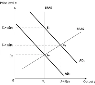
line to right from AD0 to AD1 as depicted in figure 1a below. It is followed by an increase in
prices (from p0 to, say, p1=(1+γ1)p0) like in output (from y0 to, say, y1=(1+λ)y0). The economy
moves along the positively sloped SRAS line in the short run from E0 to the transitory
[image:17.595.135.439.456.727.2]equilibrium E1.
Figure 1a. A positive demand shock in the AS-AD model
E2
E1
E0
0 (1+γ2)p0
(1+γ1)p0
p0
(1+λ)y0
y0
SRAS
AD1
AD0
LRAS
17
As time passes, however, inflation expectations adjust so that AS becomes vertical (see LRAS
on the figure) and the economy moves along the new AD1 line from E1 to its new long-run
equilibrium E2. The domestic production returns to its natural level y0 while there is an
additional inflationary impact pushing the price level to p2=(1+γ2)p0.
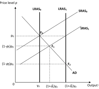
However this picture may be completed when considering the response of price and output
to a permanent shock from the supply side as it can be seen on figure 1b below. If again
positive, domestic activity will automatically rise from y0 to y1=(1+δ1)y0, and finally to reach
a higher natural level y2=(1+δ2)y0. Instead, price should fall gradually to p1=(1-δ1)p0. Starting
at point F0 on figure 1b, adjustments in production and prices will continue until the
stationary state F2 is met at the intersection of the AD curve with the new long-run AS line
[image:18.595.116.452.432.734.2]LRAS1.
Figure 1b. A positive demand shock in the AS-AD model
(1+δ2)y0
SRAS1
F2
F1
F0
0
(1-ϕ2)p0
(1-ϕ1)p0
p0
(1+δ1)y0
y0
SRAS0
AD LRAS0
Output y
Price level p
18
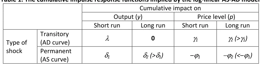
All these effects imply specific features of the impulse response functions built from the
structural vector autoregression extracted from a reduced form like (1). These are
[image:19.595.70.524.226.340.2]summarized in the following table 1.
Table 1. The cumulative impulse response functions implied by the log-linear AS-AD model
Cumulative impact on
Output (y) Price level (p)
Short run Long run Short run Long run
Type of shock
Transitory
(AD curve) λ 0 γ1 γ2 (>γ1)
Permanent
(AS curve) δ1 δ2 (>δ1) –ϕ1 −ϕ2 (<–ϕ1)
Note: All Greek letters refer to positive coefficients.
If the long-run neutrality hypothesis is valid, and provided that the AS and AD relationships
are linear, their respective slope coefficients can be recovered as:
.
, 2 1
1
λγ γ η λ
γ η
− − =
= AD
AS and (26)
In practical terms, knowledge of the cumulative IRFs to a transitory shock is sufficient to
determine the values of the above ratios. BE (1994) give a nice illustration of the economic
meaning of these functions. But they do not go on further to determine precisely the slope
parameters. On these grounds, one may be interested in comparing (26) with (19) and (22).
Table 1 also reveals another possible identification strategy for the VAR, inspired by
Uhlig’s (2005) “agnostic” approach. As it stands, sign-restrictions on the impulse response
functions can be easily inferred from this basic macroeconomic setting. Positive demand
shocks and cost-push disturbances indeed exert opposite effects on the price level on impact
(compare fig. 1a and fig. 1b above). The long-run neutrality constraint may be thus skipped
19
4. Empirical evidence on fixed exchange rate regimes
4.1. Data
Data are taken from the Eurostat database on a monthly basis over the period
1996:01-2008:12. The industrial production index (IPI) in volume is used as a proxy for output.
Inflation is measured on the basis of the Harmonized Consumer Price Index (HCPI). All these
variables are taken in logs. Price and output are assumed to follow I(1) processes, so that
they are first-differenced according to specification (1) above. This approach conforms to
what is usually assumed in the empirical literature on shock asymmetry under fixed
exchange rate regimes. Few of the past studies indeed run formally unit-root and
cointegration-rank tests. Bayoumi and Taylor (1995) is one noticeable exception where Engle
and Granger’s two-step procedure is applied.
In order to illustrate the previous principles findings and, in particular, to check for the
robustness of the empirical findings from the BE approach, we focus on the eleven founders
countries which joined the EMU in 1999. Greece is also included to the dataset since its
adhesion to the euro was already planned at that time. It also allows for comparing the
results for the so-called “PIIGS” with what was often considered as the core of the former
German Mark zone. Germany is taken as reference for all the bilateral comparisons since it is
20
4.2. Relative size and paths of permanent and transitory shocks
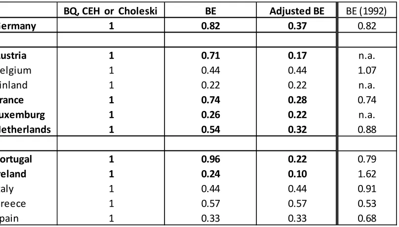
Table 2 below reports the variance ratios between the identified permanent and transitory
shocks in each country over the whole period. Each column refers to a specific procedure of
VAR identification. “BQ” refers to Blanchard-Quah’s (1989) method, “BE” to
Bayoumi-Eichengreen’s (1992), “Adjusted-BE” involves the transition matrix as given by formula (14)
in the text, and “Choleski” to the well-known approach.
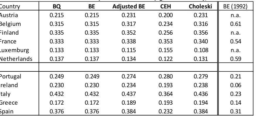
Table 2. Relative size of structural shocks under various decompositions 1996:01-2008:12
Note: Figures are ratios of the standard deviations of transitory relative to permanent shocks.The final column reports BE's (1992) initial results in terms of demand relative to supply shocks over 1962-1988.
From table 2, we conclude that non-normalized structural shocks lead systematically to
variance ratio less than unity. This means that transitory shocks are smaller than the
permanent ones. This result holds whether BE’s procedure is corrected by the transition
matrix Q or not. The only exception is Portugal where unadjusted BE’s approach leads to
permanent and temporary shocks of almost equal sizes.
BQ, CEH or Choleski BE Adjusted BE BE (1992)
Germany 1 0.82 0.37 0.82
Austria 1 0.71 0.17 n.a.
Belgium 1 0.44 0.44 1.07
Finland 1 0.22 0.22 n.a.
France 1 0.74 0.28 0.74
Luxemburg 1 0.26 0.22 n.a.
Netherlands 1 0.54 0.32 0.88
Portugal 1 0.96 0.22 0.79
Ireland 1 0.24 0.10 1.62
Italy 1 0.44 0.44 0.91
Greece 1 0.57 0.57 0.53
[image:21.595.81.485.333.563.2]21
Although all these countries belong to the same currency union, they exhibit markedly
differences regarding the shocks which hit their economies. Relying on BE’s decomposition,
the euro founder members can be divided into two groups: Germany, Austria, and France
are characterized by a variance ratio in the [0.7,1[ range like Portugal, whereas permanent
disturbances dominate by far the transitory shocks in the other Member States.
This picture conforms reasonably well to the core-periphery view of the European Monetary
Union. This picture is broadly consistent with Bayoumi and Eichengreen’s (1992) findings for
the pre-EMU period (see their reported estimates in the last column of table 2). Contrary to
these authors, demand (here transitory) shocks are less sizeable than supply (or permanent)
ones as Belgium and Ireland might have experienced in the past decades.
What is also at stake here are the economic consequences of the European monetary
unification. One can indeed hardly agree with BE’s conjecture that industrial specialization
has strengthened in the euro Members States so that demand disturbances now outweigh
those from the supply side. Rather, our estimates would give support to the alternative
“diversification” hypothesis. The European process seems to be distinct from the one
observed at the level of the US regions.
Furthermore, the choice of the transition matrix given by equation (14) may indeed matter
for assessing the size of the structural macroeconomic shocks. The corresponding estimates
reported in the last column of table 2 reveal to types of countries. The ratio of standard
deviations of shocks is left unchanged when modifying BE’s procedure in the case of
Belgium, Finland, Italy, Greece, and Spain. This contrasts with the sharp decrease
experienced by the remaining countries under study. The switch from the original BE’s
method to the proposed decomposition given by the identity (12) implies a further reduction
22
Adjusting BE’s factorization for the transition matrix Q may modify one’s view about the
way EMU actually operates. From the third column of table 2, it is uneasy to distinguish the
core from the periphery of the euro area on the sole basis of the size of domestic shocks.
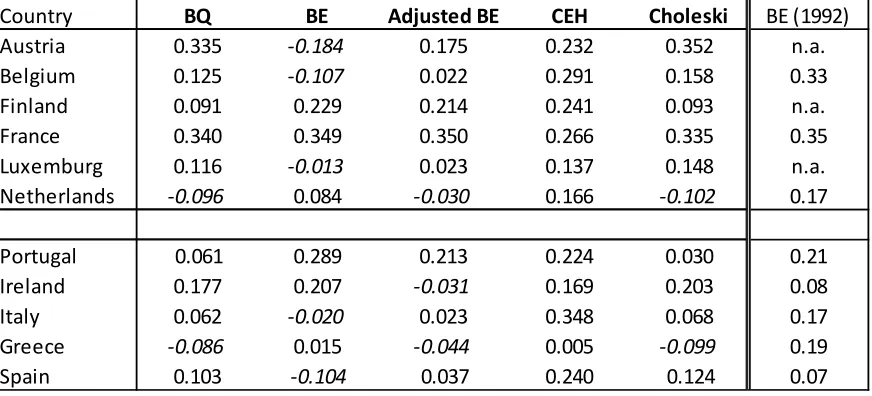
4.3. Shock asymmetries and the European currency union
Let us now consider the sensitivity of asymmetry measures to the set of identifying
restrictions. We first consider the correlation coefficients between each type, permanent or
transitory, shock. All of them are computed against Germany. Correlations between
permanent shocks are reported in table 3, those associated to temporary innovations can be
[image:23.595.77.514.435.634.2]found in table 4 below.
Table 3. Correlation coefficients of permanent shocks (against Germany, 1996:01-2008:12)
Note: The final column reports BE's (1992) initial results in terms of supply shocks over 1962-1988.
Results from table 3 illustrate the equivalence principle between BQ’s and the Choleski
decomposition scheme as demonstrated by Ribba (1997), and Fisher and Hu (1999, 2000). A
similar conclusion can be drawn from table 4 below. Because they give similar series of
Country BQ BE Adjusted BE CEH Choleski BE (1992)
Austria 0.215 0.215 0.231 0.200 0.231 n.a.
Belgium 0.315 0.315 0.317 0.234 0.316 0.61
Finland 0.335 0.335 0.352 0.256 0.356 n.a.
France 0.333 0.333 0.338 0.353 0.340 0.54
Luxemburg 0.133 0.133 0.115 0.155 0.108 n.a.
Netherlands 0.137 0.137 0.134 0.122 0.131 0.59
Portugal 0.249 0.249 0.274 0.280 0.279 0.21
Ireland 0.230 0.230 0.234 0.193 0.238 0.06
Italy 0.432 0.432 0.437 0.364 0.436 0.23
Greece 0.172 0.172 0.189 0.193 0.194 0.14
23
structural shocks country by country, the choice between these two particular sets of long-
and short-run restrictions is inconsequential for the correlation coefficients themselves.
Therefore, referring to the AS-AD framework in order to assume the long-run neutrality of
output to transitory shocks does not matter for the appraisal of stochastic asymmetry within
a currency union like the euro area. This new empirical evidence, jointly with the theoretical
results, directly challenge the common econometric practice inherited from the influential
works of Bayoumi and Eichengreen in that field.
Estimated values reported on table 3 confirm that the measurement of the correlation
between permanent shocks does not depend to the way of factorizing the covariance matrix
of the VAR residuals. Assigning unit variance to all shocks – like in Blanchard and Quah
(1989) – or allowing for structural disturbances of unequal sizes – as suggested by Bayoumi
and Eichengreen (1992, 1994) – leads to the same level of asymmetry in terms of permanent
shocks. This is well in accordance with BE’s premise: their departure to the BQ approach
should imply just a rescaling of shocks, thereby leaving their other properties unchanged.
While BQ put the emphasis on the discrepancies between the core and the peripheral
countries during the pre-EMU phase, greater homogeneity is found amid the euro founder
Members during 1996-2008. As shown on table 3, asymmetry in terms of permanent shocks
has increased in the core (Belgium, France, and the Netherlands) against Germany. At the
opposite, permanent shocks to the periphery (namely the PIIGS) seem to be more correlated
to those hitting the German economy. Based on this criterion, Greece is as far to the euro
area as other small open countries like Ireland, the Luxemburg or even the Netherlands.
Table 4 below gives the corresponding correlation estimates between transitory shocks over
the whole sample period. The equivalence principle between the BQ the Choleski
24
These are negative, though close to zero, for Greece and the Netherlands. They are of the
same order of magnitude as the asymmetry in permanent shocks only in Austria and France.
Shocks to the remaining countries are essentially idiosyncratic when they have temporary
effects on domestic output. This is more in accordance with the core-periphery view, though
it deserves some words of caution as in Bayoumi and Eichengreen (1992) (see their own
[image:25.595.75.511.306.504.2]estimates in the last column of table 4).
Table 4. Correlation coefficients of transitory shocks (against Germany, 1996:01-2008:12)
Note: The final column reports BE's (1992) initial results in terms of demand shocks over 1962-1988.
But things turn to be very different if one follows BE’s methodology. The second column of
table 4 indeed reveals that the picture about asymmetry in terms of transitory shocks is
modified. In almost all cases, correlations change of magnitude if we switch from the BQ
factorization to the (unadjusted) BE decomposition. For example, the correlation between
the Irish and the German transitory shock rises by a third roughly. It doubles at least in
Finland, and even quadruples in the Portuguese case.
If the BQ approach were viewed as the relevant one, asymmetry in the temporary
“surprises” would then be underestimated. However, we are led to the opposite conclusion
Country BQ BE Adjusted BE CEH Choleski BE (1992)
Austria 0.335 -0.184 0.175 0.232 0.352 n.a.
Belgium 0.125 -0.107 0.022 0.291 0.158 0.33
Finland 0.091 0.229 0.214 0.241 0.093 n.a.
France 0.340 0.349 0.350 0.266 0.335 0.35
Luxemburg 0.116 -0.013 0.023 0.137 0.148 n.a.
Netherlands -0.096 0.084 -0.030 0.166 -0.102 0.17
Portugal 0.061 0.289 0.213 0.224 0.030 0.21
Ireland 0.177 0.207 -0.031 0.169 0.203 0.08
Italy 0.062 -0.020 0.023 0.348 0.068 0.17
Greece -0.086 0.015 -0.044 0.005 -0.099 0.19
25
as concerns Austria, Belgium, Italy, and Spain: there is now evidence of strong asymmetries
since correlations between BE shocks turn out to be negative. There are only two Member
States – namely, France and Ireland – whose results are unaffected.
Although things remain the same in terms permanent shocks, the situation is now
completely different, if not reversed, when considering transitory disturbances. It is thus no
longer possible to conclude with Bayoumi and Eichengreen that relaxing the assumption of
equal and unitary variances would just amount to a rescaling of the innovations of the SVAR.
As demonstrated in section 2, the BE factorization is actually defined up to some
orthonormal matrix. In particular, a transition matrix Q can be found so that the structural
shocks we get by the “adjusted” BE decomposition behave like those corresponding to the
BQ procedure. This should imply similar correlation coefficients. Even though it is the case
for permanent shocks (table 3), there are noticeable discrepancies as concerns the transitory
components (table 4). The estimated value is reduced by one half or more in Austria,
Belgium, Luxemburg, Italy, and Spain. Taken in absolute values, it doubles or more in
Finland, the Netherlands, Portugal, and Greece. The equivalence prevails in France only. By
contrast, a change in the sign of the correlation coefficient is observed in the Irish case if the
BQ result is taken as a benchmark.
Though surprising at first sight, these results can be explained by the non-uniqueness of the
transition matrix as it has already been stressed in section 2. In principle, one has to pick up
one of the eight possible writings of Q given by equation (12). It is therefore easy to recover
a positive correlation for Ireland by an appropriate transformation of Q. Still, none of the
available transition matrices enables to retrieve exactly the BQ-type correlation coefficients
26
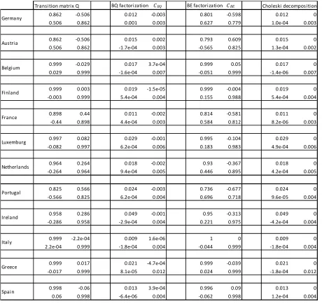
The difficulty to retrieve the BQ correlations from the “adjusted” BE factorization may lie in
the estimated transition matrices. Table 5 reports the Q matrices used to built the tables 2 to
4. It is worth highlighting that Q is close to the identity matrix in the vast majority of cases.
Off-diagonal elements seem to be highly sensitive to, even small, departures from unity on
the principal diagonal of this type of rotation matrix. But the cases of Austria and Portugal
are left unexplained.
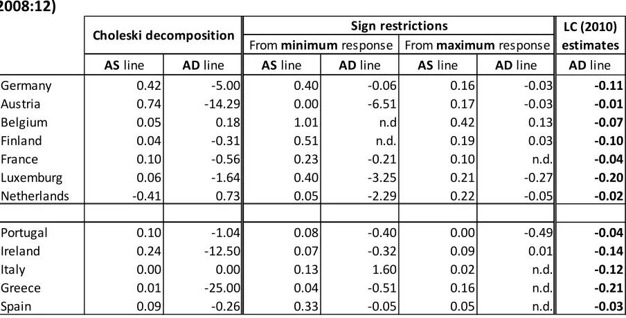
4.4. Responses to shocks and the underlying AS-AD model
The evidence about slope estimates of the aggregate supply function is rather mixed when
the CEH identification strategy is employed. Table 6 below reports the corresponding figures
for the founder members of the euro area during 1996-2008. According to the above system
(15), the slope parameter for the AS curve is given by 1/α. Positive excepted values are
reported in bold face. For comparison purposes, the results obtained by Lee and Crowley
(2010) for the same group of euro Members are shown in the last column of this table.
[image:27.595.72.528.583.752.2]These come from a New Keynesian model augmented by a Taylor rule followed by the ECB.
Table 6. Slope estimates of AS curves under CEH identifying restrictions (1996:01-2008:12)
Lag-order p
of the VAR 1 2 3 4 5 6 7 8 9 10 11 12
LC (2010) estimates
Germany -0.27 -0.16 -0.19 -0.58 -0.78 -2.38 0.70 0.58 0.76 0.63 0.87 -0.04 0.02
Austria 0.01 -0.04 -1.41 -0.16 0.07 0.03 0.02 0.04 0.08 0.04 -0.02 -0.10 0.10
Belgium 5.56 6.67 -3.85 -3.70 -25,00 0.03 0.16 0.25 0.26 0.27 0.32 0,00 0.26
Finland 33.33 0.15 0.24 0.50 0.38 0.18 0.04 0.03 0.13 0.16 0.06 -0.12 0.05
France 0.28 0.05 0.05 -0.23 -1.10 -0.30 0.04 0.04 0.08 0.04 -0.03 -0.11 0.23
Luxemburg -1.49 -1.09 -0.81 -1.11 -3.13 50.00 0.13 0.16 0.30 0.12 0.10 0.01 0.05
Netherlands 1.37 0.49 -1.12 -0.71 -2.70 0.50 0.03 0.71 0.56 0.51 -0.09 -0.44 0.13
Portugal 0.44 0.10 -0.08 -0.20 -0.07 0.02 -0.08 -0.21 -0.47 -0.26 -0.27 0.10 0.06
Ireland -0.37 -0.22 -0.09 -0.10 -0.25 1.19 0.04 -0.20 -0.23 -0.49 0.00 1.85 0.07
Italy -684.93 -1.32 -1.12 -2.27 -2.63 0.30 0.24 0.36 0.36 0.54 0.46 -0.04 0.13
Greece 0.37 -11.11 -5.00 -4.55 -5.00 -0.63 -0.83 5.26 1.59 1.43 2.08 0.18 0.47
27
The slope estimates with the CEH approach exhibit considerable variability with the chosen
lag-order of the VAR system. Adding just one more lag to the dependent variables may lead
to either a sudden change in the order of magnitude or to a sign reversal, as it is observed in
all the countries under study. As concerns Austria, the parameter α varies from -26.32 to
151.29 when it is computed as in (19). Nine lags in the vector autoregression give the least
unreasonable value of 12.2. This leads to an AS slope coefficient of 0.08 close to Lee and
Crowley’s (LC, 2010) result. There is thus evidence of relatively flat AS curves in the founders
of the euro area.
Discrepancies are observed between the CEH SVAR approach and the LC New Keynesian
model. These are particularly sharp in the German case, our reference country for the
bilateral comparisons. More seriously, it appears from table 6 that the German Phillips curve
is steeper than in France, contrary to the empirical evidence from New Keynesian DGSE
models (e.g. Brissimis and Skotida (2008) among others).
This may be explained by the ECB’s commitment to an interest rate policy rule which is
accounted for in these general equilibrium models. In addition, the slope coefficient of the
AD curve is left unconstrained. It proves to be systematically lower than unity and to vary
amid the euro Member States. Lee and Crowley (o. p.) reports values ranging from 0.01 to
0.21. This is inconsistent with the full price indexation hypothesis made by CEH (2006). If the
bivariate VAR setting is misspecified, there may well be strong bias in the parameter
estimates as well as in the impulse response functions (see Braun and Mittnick, 1993). This is
a crucial issue since α comes from the long-run dynamic multipliers.
Table 5 also shows that implausible (negative) values of the AS slope are usually obtained
with small lags in the vector autoregression. Estimates of α are also much more sensitive to
28
VAR process. Worrying about parsimony, the econometrician often relies on standard
information criteria, especially Schwartz’s conservative one, to get an “optimal” value for p.
The “best” value is often 1, rarely 2, as it is the case in the estimated VARs underlying the
building of tables 2 to 4. But, as it is apparent here, this choice may be viewed as too
conservative if one follows the CEH procedure of VAR identification. Unreliable estimates of
the slope of the AS curve would then be obtained.
As already pointed out by Braun and Mittnick (1993), adding lags to the autoregressive
component of the dynamic system may circumvent (at least part of) the misspecification
problems to recover the true impulse response functions. As regards the CEH approach, it
may be reflected in an severe biased estimate of the slope parameter of the AS curve. This
may be due to omitted moving average terms which often appear in a New Keynesian
framework under the rational expectation hypothesis. They are clearly neglected in “pure”
VAR reduced forms like (1).
Slope estimates based on the graphical representation of the AS-AD model are reported on
with each other: the BQ strategy as depicted in table 1 and Uhlig’s pure sign approach.
According to the first method, the estimated coefficients have the expected sign in almost all
cases. A major exception is Netherlands for which the identified shocks can hardly be
interpreted as supply and demand disturbances because of the complete sign reversal in
their observed effects on output and prices. As concerns Belgium, its AD curve seems also to
be positively sloped, contrary to what the inflation–unemployment tradeoff would have
implied. Another striking feature is that the strong heterogeneity in the implied slope values
when the long-run neutrality of output is assumed. AD curves are generally found to be
steeper than AS curves, reaching unrealistic levels in the core (Austria and Germany) like at
29
the findings of other recent studies (see last column of table 6 above). Instead, AD slope
parameters exhibit strong discrepancies with Lee and Crowley’s (2010) values (see the last
[image:30.595.76.524.199.432.2]column of table 7).
Table 7. Slope estimates from the graphical view of the AS-AD model (1996:01-2008:12)
Note: Undetermined values of slope parameters are abbreviated with n.d..
If we switch to the agnostic approach, results differ markedly. Remember that the estimates
of slope coefficients are now obtained from impulse response functions based on the VAR in
levels. The values given by the pure sign approach are computed according to formulas in
table 1 from the impulse response functions shown on graphics 2 and 3 in the annex. Sign
restrictions were imposed output and price responses during the next 3 months following a
transitory (demand) shock. 500,000 simulations have been launched of which at most
50,000 “successes” have been collected. The range of effects is revealed by the minimum
and maximum impacts on each of these aggregates over a five-year horizon (or equivalently
AS line AD line AS line AD line AS line AD line AD line
Germany 0.42 -5.00 0.40 -0.06 0.16 -0.03 -0.11
Austria 0.74 -14.29 0.00 -6.51 0.17 -0.03 -0.01
Belgium 0.05 0.18 1.01 n.d 0.42 0.13 -0.07
Finland 0.04 -0.31 0.51 n.d. 0.19 0.03 -0.10
France 0.10 -0.56 0.23 -0.21 0.10 n.d. -0.04
Luxemburg 0.06 -1.64 0.40 -3.25 0.21 -0.27 -0.20
Netherlands -0.41 0.73 0.05 -2.29 0.22 -0.05 -0.02
Portugal 0.10 -1.04 0.08 -0.40 0.00 -0.49 -0.04
Ireland 0.24 -12.50 0.07 -0.32 0.09 0.01 -0.14
Italy 0.00 0.00 0.13 1.60 0.02 n.d. -0.12
Greece 0.01 -25.00 0.04 -0.51 0.16 n.d. -0.21
Spain 0.09 -0.26 0.33 -0.05 0.05 n.d. -0.03
From maximum response From minimum response
Sign restrictions
Choleski decomposition LC (2010)
[image:30.595.74.526.206.436.2]30
60 months). For ease of comparisons, the response functions derived from the Choleski
decomposition are also reported on these graphics.
The estimates for AS curves are close to those reported on table 6 in a majority of countries.
As emphasized by the previous studies, AS like AD curves are very flat. Our results do not
give support to the full price indexation assumption made by CEH (2006), even a statistical
test cannot be put formally. Table 7 also shows the difficulties in calculating the slope the
aggregate demand relationship. These are sometimes impossible to determine or wrongly
signed because the impulse response function of industrial production to a transitory shock
does not conform to what is expected from the AS-AD model.
5. Conclusion
This paper has discussed the relevance of long-run restrictions in structural VAR models
within the textbook AS-AD theoretical framework. As popularized by Bayoumi and
Eichengreen (1992, 1994), the latter is often used as the economic background to investigate
the empirical properties of shocks under alternative exchange rate agreements. Our
contribution in this field is twofold.
As regards structural VAR modeling, it is shown how Blanchard and Quah’s (1989) stratregy
is linked to its competing alternatives in order to distinguish permanent from transitory
shocks. In particular, it is shown how the modified procedure suggested by Bayoumi and
Eichengreen themselves may depart significantly from BQ’s. However, a transition matrix
can be found to back out BQ’s decomposition of the VAR residuals. Still, this particular
31
relaxing auxiliary assumptions in VAR identification – especially the orthogonalization of
shocks in a given country – may lead to significant departure from the BQ decomposition
scheme. Since VAR identification through long-run restrictions has been severely
questioned, short-run alternatives have also been considered here. We are thus led to
emphasize a important result which has been disregarded by the empirical literature of fixed
exchange rate regimes: zero-restrictions on either long-run or comtemporaneous responses
of variables to shocks may be strictly equivalent. As such, a Choleski decomposition is not a
alternative to BQ’s approach.
These new insights in structural VAR modeling have important consequences for the
empirical analysis of shock asymmetry under a fixed exchange rate regime. Our previous
findings have been illustrated the experience of the eleven founder members of the euro
area (plus Greece) during 1996-2008.
Taking into account the transition matrix from BE to BQ decompositions matters for
evaluating the relative size of permanent relative to transitory shocks. Though permanent
shocks always dominate, the country ranking appears to be very sensitive to inclusion of the
transition matrix to identify both sources of structural shocks. The updated evidence
provided also clearly conflicts with BE’s premise that the currency union would have
fostered industrial specialization thereby increasing the relative size of transitory (demand)
disturbances. Furthermore, linking the BE decomposition to the BQ one through the
transition seems to be inconsequential for the measurement of asymmetry in permanent
shocks, whereas it has a dramatic influence on the empirical assessment of asymmetry in the
transitory component. It is also shown that the issue raised by BE’s identification strategy is
further complicated by the non-uniqueness of the transition matrix itself. The former is
32
Given’s matrices underlying the (short-run) sign restrictions for the VAR identification. From
this perspective, the basic AS-AD diagram used by BE may help recover the slope coefficients
of the AS and AD curves. However, sign-restrictions according to Uhlig’s (2005) pure agnostic
approach give in general more reliable estimates of these slope parameters than
zero-constraints on the response functions derived from VAR estimates do. Aggregate demand
and well supply curves are usually found to be flat, but they differ substantially from one
euro Member State to another.
From this perspective, the conclusions drawn from our analysis may also have implications
to other important economic issues. Similar concerns about structural VAR modeling can
indeed be found in the business cycle literature where the characterization of the underlying
dynamic stochastic (general equilibrium) model plays a crucial role (Canova (2009)). The
identification problem should deserve further analysis since it is also involved in monetary
33
Bibliography
Alessi A., Barigozzi M. and Capasso M. (2009). “Nonfundamentalness and identification in
structural econometric models: a review”, mimeo, November.
Bayoumi T. and Eichengreen B. (1992). “Shocking aspects of European monetary
integration », in F. Torres and F. Giavazzi (eds.), Adjustment and Growth in the European
Monetary Union, Cambridge University Press, New York, pp. 193–292.
Bayoumi T. and Eichengreen B. (1994). “Adjustment under Bretton Woods and the
Post-Bretton-Woods float: an impulse-response analysis”, Economic Journal, 104(425), 813-27.
Bayoumi T. and Taylor M. (1995). “Macro-economic shocks, the ERM, and tri-polarity”,
Review of Economics and Statistics, 77(2), May, 321-31.
Bergman M. (2005). “Do long-run restrictions identify supply and demand disturbances?”,
mimeo, October.
Blanchard O. and Quah D. (1989). “The dynamic effects of aggregate demand and supply
disturbances”, American Economic Review, 79(4), September, 655-73.
Blanchard O. and Quah D. (1993). “The dynamic effects of aggregate demand and supply
disturbances: Reply”, American Economic Review, 83(3), June, 653-8.
Braun P. and Mittnick S. (1993). “Misspecifications in vector autoregressions and their
effects on impulse responses and variance decompositions”, Journal of Econometrics, 59,
319-41.
Brissimis S. and Skotida I. (2008). “Optimal monetary policy in the Euro area in the presence
of heterogeneity”, Journal of International Money and Finance, 27(2), 209-26.
Canova F. (2009). “How much structure in empirical models?”, chapter 2 in T. Mills and K.
34
Cooley T. and Dwyer M. (1998). “Business cycle analysis without much theory. A look at
structural VARs”, Journal of Econometrics, 83, 57-88.
Cooley T. and LeRoy S. (1985). “Atheoretical macroeconometrics. A critique”, Journal of
Monetary Economics, 16, 283-308.
Cover J., Enders W. and Hueng C. (2006). “Using the aggregate demand-aggregate supply
model to identify structural demand-side and supply-side shocks: results using a bivariate
VAR”, Journal of Money, Credit, and Banking, 38(3), April, 777-90.
Crowder J. (1995). “The dynamic effects of aggregate demand and supply disturbances.
Another look”, Economics Letters, 49, 231-7.
Faust J. and Leeper E. (1997). “When do long-run identifying restrictions give reliable
results?”, Journal of Business & Economic Statistics, 15, July, 345–53.
Fidrmuc, J. and Khoronen I. (2006). “Meta-Analysis of the Business Cycle Correlation
between the euro Area and the CEECs”, Journal of Comparative Economics, 34 (3), 518-37.
Fisher L. and Hu H.-S. (1999). “Weak exogeneity, and long-run and contemporaneous
identifying restrictions in VEC models”, Economics Letters, 63, 159-65.
Fisher L., Hu H.-S., and Summers P. (2000). “Structural identification of permanent shocks in
VEC model: a generalization”, Journal of Macroeconomics, 22(1), 53-68.
Fry R. and Pagan A. (2009). “Sign restrictions in structural vector autoregressions: a critical
review”, mimeo, December.
Keating J. (2009). “When do Wold orderings and long-run recursive identifying restrictions
yield identical results?”, mimeo, University of Kansas.
Lee J. and Crowley P. (2010). “Evaluating the Monetary Policy of the European Central Bank”,
35
Lippi F. and Reichlin L. (1993). “The dynamic effects of aggregate demand and supply
disturbances. Comment”, American Economic Review, 83(3), 644-52.
Pagan A. and Pesaran H. (2008). “Econometric analysis of structural systems with permanent
and transitory shocks”, Journal of Economic Dynamics and Control, 32, 3376-95.
Quah D. (1995). “Misinterpreting the dynamic effects of aggregate demand and supply
disturbances”, Economics Letters, 49, 247-50.
Ribba A. (1997). “A note on the equivalence of long-run and short-run identifying restrictions
in cointegrated systems”, Economics Letters, 56, 273-76.
Rubio-Ramirez J., Waggoner D. and Zha T. (2010). “Structural vector autoregressions: theory
36
[image:37.595.72.532.187.621.2]Annex
Table 5. Factorizations of the covariance matrix of the VAR residuals and the transition
matrix between the BE and BQ decompositions
Transition matrix Q BQ factorization CBQ BE factorization CBE Choleski decomposition
0.862 -0.506 0.012 -0.003 0.801 -0.598 0.012 0
0.506 0.862 0.001 0.003 0.627 0.779 1.0e-04 0.003
0.862 -0.506 0.015 0.002 0.793 0.609 0.015 0
0.506 0.862 -1.7e-04 0.003 -0.565 0.825 1.3e-04 0.002
0.999 -0.029 0.017 3.7e-04 0.999 0.05 0.017 0
0.029 0.999 -1.6e-04 0.007 -0.051 0.999 -1.4e-06 0.007
0.999 0.003 0.019 -1.5e-05 0.999 -0.004 0.019 0
-0.003 0.999 5.4e-04 0.004 0.155 0.988 5.4e-04 0.004
0.898 0.44 0.011 -0.002 0.814 -0.581 0.011 0
-0.44 0.898 4.4e-04 0.003 0.584 0.812 8.2e-06 0.003
0.997 0.082 0.029 -0.001 0.995 -0.104 0.029 0
-0.082 0.997 6.2e-04 0.006 0.183 0.983 4.9e-04 0.006
0.964 0.264 0.018 -0.002 0.93 -0.367 0.018 0
-0.264 0.964 9.4e-04 0.005 0.446 0.895 4.2e-04 0.005
0.825 0.566 0.024 -0.003 0.736 -0.677 0.024 0
-0.566 0.825 6.2e-04 0.004 0.696 0.718 9.6e-05 0.004
0.958 0.286 0.049 -0.001 0.95 -0.313 0.049 0
-0.286 0.958 -2.9e-04 0.004 0.221 0.975 -4.2e-04 0.004
0.999 -2.2e-04 0.009 1.6e-06 1 0 0.009 0
2.2e-04 0.999 -1.8e-04 0.004 -0.044 0.999 -1.8e-04 0.004
0.999 0.017 0.021 -4.7e-04 0.999 -0.039 0.021 0
-0.017 0.999 8.1e-05 0.012 0.024 0.999 -1.8e-04 0.012
0.998 -0.06 0.013 3.9e-04 0.996 0.09 0.013 0
0.06 0.998 -6.4e-06 0.004 -0.062 0.998 1.2e-04 0.004
Netherlands
Portugal
Ireland
Italy
Greece
Spain Germany
Austria
Belgium
Finland
France