Munich Personal RePEc Archive
When does variety increase with quality?
Basov, Suren and Danilkina, Svetlana and Prentice, David
La Trobe University, University of Melbourne
2 February 2009
Online at
https://mpra.ub.uni-muenchen.de/29708/
When does variety increase with quality?
Suren Basov
∗, Svetlana Danilkina
†, and David Prentice
‡March 19, 2011
Abstract
Casual empiricism suggests higher quality is associated with greater variety. How-ever, recent theoretical and empirical research has either not considered this link, or has been unable to establish unambiguous predictions about the relationship between quality and variety. In this paper we develop a simple model, which predicts that for low qualities variety should be positively correlated with quality and we establish conditions under which variety will either increase or decrease with quality at higher quality levels. The producer uses variety to increase the profitability of price discrim-ination across different qualities, by increasing the likelihood consumers choose high price products among products yielding the same utility. We show that the number of varieties offered by the monopolist is greater than the social optimum. The predictions of the model are supported by an empirical analysis of the market for cars. A wide range of car manufacturers are found to offer a hump-shaped distribution of varieties.
∗School of Economics and Finance, LaTrobe University, Bundoora, Victoria 3086, Australia,
[email protected]. Thanks to Catherine de Fontenay, Tue Gørgens, Phillip Leslie, Phillip McCalman and Lawrence Uren for helpful comments. This research is supported by ARC Discovery Grant DP0881381 “Mechanism design under bounded rationality: The optimal contracts in the complex world.”
†Department of Economics, The University of Melbourne, Melbourne, Victoria 3010, Australia,
‡School of Economics and Finance, LaTrobe University, Bundoora, Victoria 3086, Australia,
1
Introduction
A casual look at the shelves of a supermarket or at producer web sites reveals that many
goods come in multiple “flavors” as part of a product line. Moreover, higher quality products
often have a larger number of flavors. Branded products almost always have more varieties
than generics. For example, there are many more varieties of the premium Pickwick tea
than of a basic Lipton brand. Furthermore, we demonstrate in this paper that this also
holds for most of the product lines offered by car manufacturers. This phenomenon is not
explained by the extensive theoretical literature examining the interaction between quality
and variety in imperfectly competitive markets where consumers’ tastes are differentiated
along one vertical dimension, quality, and one horizontal dimension, flavor.1 In such models
the correlation between quality and variety depends on the way they enter the consumer’s
utility function, their joint distribution, and the market structure. Therefore, it is impossible
to come up with unambiguous predictions suitable for estimation or testing.
Recent work by Draganska and Jain (2005) models varieties, in product-lines, as
hori-zontal differentiation but does not explicitly consider vertical differentiation highlighted in
models of price discrimination. Hence, the link between quality and variety is not analyzed.
We adapt a standard probabilistic choice model to demonstrate there tends to be a
positive relationship between quality and variety. In the model, a second degree
price-discriminating monopolist offers a menu of products of increasing quality. Consumers,
mod-elled as caring about quality, but indifferent between flavors of the same quality, respond by
randomizing across products offering the same utility. The monopolist increases the
prof-itability of price discrimination by offering more flavors at higher qualities. This increases
both the likelihood consumers choose high-price products when randomizing and the
ex-pected profits. However, if the market is thin at high quality levels, the profit maximizing
number of varieties falls again. In this case, the distribution of varieties is hump shaped.
These predictions are tested using data on the product-lines of seventeen large
tional car companies in the Australian market. We perform a dip test to determine most
makes have a unimodal distribution of varieties. Most of the remaining makes are shown to
have one large mode. We then estimate the flexible beta density functions for each make and
conclude the densities for most makes are both unimodal and hump-shaped. It is notable
this holds for makes from the discount to the premium end of the market. To determine if
this pattern of varieties is an example of flavor proliferation, we test if the distribution of
varieties offered is statistically significantly different from that consistent with the
distribu-tion of demand. A set of Kolmogorov-Smirnov tests suggest the distribudistribu-tion of varieties and
demand differ for all but the cheapest makes in a way consistent with flavor proliferation.
One might object that most consumer product markets, including cars, are oligopolistic
rather than monopolistic. However, the model can be generalized to this case along the lines
of Champsaur and Rochet (1989). It can be shown that under some reasonable conditions
there exists an equilibrium, where each producer specializes on a particular range of qualities.
Qualitatively, the outcome is similar to the monopoly outcome. Proliferation of varieties in
the oligopolistic case will be due to two effects: competition between the producers and
price discrimination between consumers of different types who buy from the same producer.
We find it interesting from the theoretical perspective that the second effect alone can lead
to strong excessive flavor proliferation even if a consumer’s choice is almost completely
determined by the vertical characteristics of the product.
This paper makes two main contributions to the literature. First, the model provides
a new explanation for observing different types of correlations between quality and variety.
These correlations result from firms attempting to price discriminate rather than, as assumed
earlier, solely from the distribution of preferences or costs — hypotheses that are notoriously
difficult to test. Second, the generality of the hump-shaped distribution of varieties offered
within the car market suggests similar distributions of product varieties may occur in other
markets. Finally, also we show that the monopolist can produce a greater than optimal
randomness in consumer behavior.2 Most existing literature tends to find that the number
of varieties produced by a monopolist tends to be less than optimal (Lancaster, 1990).3
The paper is organized in the following way. In Section 2 we provide some preliminary
evidence to demonstrate a link between quality and variety for the car market. In Section 3 we
introduce the simplest possible probabilistic choice model of consumer behavior with which
to analyze the effect of increasing product variety on the profitability of price discrimination
– the Luce model (Luce, 1959). The section closes by introducing the concept of a nearly
deterministic consumer. In Section 4 we demonstrate that in a world populated by nearly
deterministic consumers, the profitability of price discrimination will be lower compared with
that predicted by the standard two-type screening model with fully deterministic consumers.
In Section 5 we propose a way to overcome this problem by introducing multiple flavors for
each quality level. In Section 6 we extend the model of Section 5 to multiple types and
generate predictions about the relationship between quality and variety. Section 7 empirically
analyzes these predictions using data from the Australian car market. Section 8 concludes.
2
Model proliferation in the car market
In this section, we provide some preliminary evidence on flavor proliferation from the car
market. A comparison of luxury, medium and small models of cars demonstrates there are
relatively more types of luxury cars on offer despite luxury cars sales being less than 10%
of the market. We then argue that this pattern is not obviously explained by differences in
profitability in the different segments of the market.
Our dataset is composed of the price and characteristics for all cars sold as new in
Aus-tralia in 1998, and registrations (sales) for cars, aggregated by model or make, for AusAus-tralia
in 1998.4 Both data sets are compiled by a private data-collection firm, Glass’s Guide.
2One should distinguish between excessive variety for agiven quality predicted by this paper and larger
than optimal product line predicted by standard screening models (e.g. Mussa and Rosen, 1978). These models do not have any horizontal variety, while the vertical size of the product line in these models is the same as in our model.
Cars in the Glass’s data set are classified by the make and the model, e.g. Toyota is
a make and Corolla is a model. Our data set of prices and characteristics contains one
observation for each distinct car offered for sale (hereafter called a variety). Though we
analyze this data set in more detail in Section 7, for now we compare, in Table 1, averages
for three groups of car models, as classified by Glass’s Guide, representing three different
levels of quality: small, medium and luxury.
The first two columns of the first panel of Table 1 summarize, for each group, the average
number of features and average price in Australian dollars.5 The consistent ranking in
terms of number of features and price suggests the ordering of these groups is broadly
consistent with ranking by quality. In general, we will consider quality in terms of the cars
characteristics, such as the size, fuel efficiency, safety and range and type of features, so to be
able to make comparisons across different types of cars. Though specific sets of consumers
may have strong preferences for specific sets of features (like smaller cars for easier inner city
parking), in general it appears that quality, as reflected by consumers’ willingness to pay, is
highly correlated with these measures.
The third column, reporting the average number of registrations (sales) by group
demon-strates that luxury car sales are less than 10% of total sales and just one fifth those of the
other two groups. It is important to keep in mind when considering alternative explanations
for flavor proliferation we document more extensively in section 7 whether they are likely to
generate so many varieties for such a small number of sales.
The last three columns report the number of makes, models and varieties for each class.
Note that the luxury class features the largest number of makes and models. It also makes
up 40% of the varieties for new cars, despite making up less than 10% of registrations.
The second panel of Table 1 confirms what is suggested in the first panel. The first three
columns report the number of registrations per make, model and variety. These numbers
are consistently lowest for the luxury class. The last two columns report the number of
models and varieties per make. The number of models per make for luxury cars is more than
twice the number for medium cars and more than 1.5 the number for small cars. This is
consistent with our focus on a positive relationship between quality and variety. The number
of varieties per make is greater for the medium and small cars than for luxury cars though.
This could either reflect thinner demand at higher prices or greater numbers of cars being
made to order relative to the other classes. That being said, it is still striking that when
so few luxury cars are sold that the numbers of varieties per make is still comparable with
those for the medium and small classes.
In Table 2, we demonstrate that these patterns occur not only across firms but within
firm product lines. We select all firms with models included in at least two of the three
groups. Then, for each group, for each firm, we calculate the average price, the average
number of features and the average number of varieties per registration. We then calculate
the ratio of the average for medium compared with small, luxury compared with medium
and, for a few makes that do not offer medium models, the ratio of luxury compared with
small. Finally we take the average of the ratios across the firms and report these averages in
Table 2. For example, for the nine makes that offer both medium and small cars, on average,
medium cars are 46% more expensive and have 69% more features than small cars. And for
each car sold there are 21% more varieties per medium car than per small car sold.
In general, the pattern of prices and features across these groups are consistent with those
in Table 1. But Table 2 also demonstrates flavor proliferation by firms. First, note that on
average, the ratio of the varieties per registration for higher quality to lower quality models
for luxury and medium models is greater than one. In other words, luxury and medium
models have, on average, more varieties per sale than lower quality models offered by the
same firm. Strikingly, there are far more varieties per registration for luxury cars relative to
medium cars than luxury cars relative to small cars if the firm does not offer any medium
cars. This is consistent with flavor proliferation to price discriminate for a firm would not
The simplest explanation for flavor proliferation is that firms offer more varieties of more
profitable cars. Hence, more varieties of luxury cars are offered than medium cars because
these cars are more profitable. Specifically, profit margins on luxury cars will be greater
than other cars if their buyers are less price sensitive as they are more interested in getting
a car with the right combination of characteristics. A related argument is that purchasers of
higher quality cars may also have more distinctive preferences that support more varieties.
This is supported by the estimated profit margins on different models of cars reported by
Berry et al. (1995). These largely increase with price, with the most expensive model they
report, the BMW 735i, also having a much larger markup than the others.
However, profitability is determined by sales as well as the markup and, as Table 1,
demonstrates, the sales of luxury models are just one fifth the sales of the small and medium
groups of cars. It seems unlikely that there is not similar distinctiveness of tastes among
the 45% of consumers that each purchase small and medium cars than the 10% purchasing
luxury cars. The estimates of Berry et al (1995) also do not support luxury cars being more
profitable, despite their higher profit margins. Amongst, the models they report, variable
profit does not generally simply increase with price. In fact, the BMW 735i has lower
estimated variable profits than most of the medium and small cars they consider. And this
does not include development costs, which are likely to be much higher for higher quality cars,
which would further reduce their profitability. In general, it is not immediately obvious that
the profit margins are sufficiently high on luxury cars to overcome much smaller sales and
greater development costs, so to make them sufficiently profitable to explain the relatively
large number of varieties relative to lower quality cars.
3
Consumer Behavior
In this section we develop a probabilistic choice model of consumer behavior to analyze
the implications of introducing new varieties of a differentiated product. The seminal book
probabilistic choice. Drawing on their work, we argue, in an online appendix, that under
reasonable conditions, one can move freely between these different interpretations of
proba-bilistic choice models for a fixed set of alternatives. The most important difference between
the models, for our purposes, is the simplicity of modelling the change in probabilities if new
alternatives are introduced. As we are agnostic about the source of probabilistic choice, for
expositional simplicity we use the Luce model, also known as the logit model, which provides
the simplest framework incorporating this feature. The first advantage of the Luce model is
that choices between varieties depend solely on the utilities associated with each variety. The
second feature, and the main property that drives our results, is that adding new varieties
leads to a strict decrease in the probabilities of choosing all previously available varieties.
The logit model has been extensively criticised on theoretical and empirical grounds
for this feature. However, the properties of the logit model we utilize are only a little
stronger than the one that necessarily arises in random-utility models, which requires that
the probabilities of existing varieties are non-increasing if new varieties are added. Finer
properties of the model, which are the focus of recent critiques, are not important for our
results. For empirical work, several alternative approaches have been proposed at least some
of which are motivated by allowing for unobserved product or consumer heterogeneity. In
the theoretical analysis, we simplify things by ignoring such heterogeneity. Furthermore as
we do not directly estimate the theoretical model but use it to motivate some tests of its
implications, if such heterogeneity is important in our application then it just biases against
finding evidence in favour of our model. After reviewing this model in the first subsection, in
the second subsection we introduce a concept of near-deterministic behavior, that specifies
the very small degree of randomness in consumer behavior required for our results.
3.1
The Luce model
In this subsection we present a simple probabilistic choice model, Luce’s (1959) logit
model, that incorporates the main property required for our results. We stress that the
required for our main theoretical results is that adding a new alternative strictly decreases
the choice probabilities of all previously accessible alternatives. The Luce model incorporates
this feature in a particularly clear way. Furthermore, it has the simplifying feature that the
choice probabilities depend solely on the utilities of the different alternatives. The choice
probabilities have the following form:
pi =
exp(ui/λ) n
X
j=1
exp(uj/λ)
. (1)
Note that the Luce model implies any two alternatives with the same utility are selected
with the same probability. Assuming identical probabilities makes the subsequent analysis
relatively simple. Relaxing this assumption only changes the results quantitatively, not
quali-tatively. In this model parameterλ, which can take values from zero to infinity, can be given
several different interpretations. For example, it may reflect the degree of randomness in
preferences due to bounded rationality or random fluctuations in preferences. Alternatively,
it can also represent the degree of horizontal differentiation of tastes. Ifλ →0 then
lim
λ→0pi =
1/k, if ui = max{u1, ....un}
0, otherwise , (2)
where integer k is the cardinality of the set of the utility maximizers.6 Note that this is
the first sense in which consumers randomize and that the probability of each choice falls as
the number of optimal varieties increases. It is also important to note that this is the main
feature of the Luce model that we use for our results. Other features of the model, which
have been recently criticized, are not essential for our results.
If λ is greater than zero, then the probability of the consumer choosing a product other
than the one that maximizes the non-random or vertical component of utility is positive.
This is the second sense in which the consumers randomize across products. For λ < ∞
the probability of choosing a product increases with the utility provided. At the extreme
6Since a fully deterministic consumer or a consumer that does not have any horizontal preferences
case where λ → ∞ the choice probabilities converge to 1/n, i.e. the choice becomes totally
random and independent of the utility level. Again, the probability of choosing each product
falls as the number of varieties increases. Note that the logit formulation is not required for
λ to play this role; for example, a probit formulation is also feasible.
3.2
A concept of a nearly deterministic consumer
In this subsection we introduce the concept of a nearly deterministic consumer — which
states that the randomness in consumer choice required to yield our results is relatively
small, corresponding to a small value of λ. Assume that the probability of different choices
by the consumer is given by a continuously differentiable function:
p(·) :Rn×R+→∆n, (3)
such that ui = uj implies pi(u, λ) = pj(u, λ) and p(u,0) is given by equation (2). Luce
probabilities, as in equation (1), satisfy these properties though the exact form of function
p(·, λ) is not important for our purposes.
Let M be the set of the utility maximizers, i.e.
M ={ui :ui = max{u1, ....un}}. (4)
Take any uj ∈M and define
∆ = min
uk /∈M
(uj −uk). (5)
Definition 1 An economic agent whose choice probabilities are given by equation (3) is
called nearly deterministic if λ <<∆.
In words, the definition says that an economic agent is nearly deterministic if λ is much
smaller (sign << reads “much smaller”) than the difference in utility between the optimal
and the next to the optimal choice. The exact meaning of “much smaller” depends on the
extent of randomness to be permitted in decision-making.
Assume that consumers differ in their preferences for quality, i.e. are different types. A
each product will be targeted for a certain type of consumer. In the standard model of price
discrimination with fully deterministic consumers infinitely small price changes can be used
to get each type of consumer to purchase the product designed for them. Introducingλ >0
mutes the effect of price changes on the probability of choice, but we require only a small
degree of randomness to obtain our results.
4
The monopolistic screening model
Let us briefly review the basic screening model with fully deterministic consumers7 and
discuss the consequences of offering the second best contract to nearly deterministic
con-sumers. Assume a risk neutral monopolist produces a unit of good with quality x at a
cost C(x), where C(·) is a strictly convex, twice differentiable function. Preferences of a
consumer, of type θ, over a unit of good with quality x are given by a twice continuously
differentiable utility functionu(θ, x). Preferences of the consumer are quasilinear in money:
v(θ, x, m) =u(θ, x) +m.
Each consumer wants to buy at most one unit of the monopolist’s goods. Type θ is private
information of the consumer. If the consumer does not purchase a good from the monopolist,
she receives utility u0(θ). For simplicity assume it does not depend on type and normalize
it to be zero. Finally, assume
u1 >0, u2 >0, u12>0.
(Here ui is the derivative of u w. r. t. the ith argument, u12 is the cross partial derivative
with respect to θ and x). The last of these conditions is known as the Spence-Mirrlees
condition or the single-crossing property.
Let us assume that θ∈ {θL, θH}.Then the optimal qualitiesxLand xH are characterized
by:
u1(xH, θH) = C′(xH)
u1(xL, θL)−C′(xL) = 1−pHpH(u1(xL, θH)−u1(xL, θL))>0 (6)
tL=u(xL, θL)
tH =u(xH, θL)−u(xL, θH) +u(xL, θL) (7)
Note that xH is at the efficient level (no distortions at the top) andxL is below the efficient
level. At these prices high value consumers are indifferent between the two products, and
low value consumers are indifferent between purchasing the low quality product and not
purchasing at all.
To place a bound on λrequires, according to equation (5), considering the gaps in utility
between the most preferred and next preferred products for each type of consumer. For
type θH, the gap in utility between its preferred and next preferred option, equal to their
information rent, is:
I21=u(xH, θH)−tH =u(xL, θH)−tL =u(xL, θH)−u(xL, θL).
For type L, who is indifferent between purchasing xL and not purchasing, the gap in utility
to its next preferred option is:
∆IC =tH −u(xH, θL), (8)
which also measures the slack in the incentive compatibility condition for the low type.
Hence we can determine
∆ = min(I21,∆IC). (9)
From now on, we will assume that
u(θ, x) =θx. (10)
This specification of the incentive compatibility constraint for the high type together with
the condition θH > θL implies a convex relationship between price and quality:
In other words, this implies for a price discriminating firm, that prices increase more than
proportionately with quality. This is a special case of a general result that states that the
optimal tariff is convex for an arbitrary type space. Indeed, letθ ∈Ω⊂R, where Ω may be
a finite set, as in this paper, or even a more general subset of R. Given an implementable
allocationx(θ), which may but need not be optimal, define consumer’s surplus by:
s(θ) =
θ
Z
θL
x(β)dβ. (12)
This allocation is implementable by tariff 8
t(x) = max
θ (θx−s(θ)). (13)
Equation (13) implies that the tariff implementing x(·) is convex. If Ω is a finite set, the
convexity requirement is reduced to:
ti+1−ti ≥θi(xi+1−xi), (14)
where the inequality is strict as long as xi+1 >0.
Let us call the contract (6)-(7) thesecond best contract. Assume that the monopolist offers
the second best contract to nearly deterministic consumers. By the definition of a nearly
deterministic consumer, parameter λ is much less than both the high type information rent
and the slack in the low type incentive compatibility constraint. Therefore, the fraction of
high type consumers who decide not to participate or the fraction of the low type consumers
who decide to choose the high quality product is negligibly small.
On the other hand, as a result of randomizing between equally preferred alternatives,
similar to that described in equation (2), approximately half of the low type consumers
decide to stay out of the market and approximately half of the high type consumers purchase
the low quality product. This leads to a drop in the monopolist’s profits which is higher
order of magnitude thanλ. If consumers were fully deterministic, then infinitely small price
changes deal with this problem but, as we have argued, infinitely small price changes will
not be sufficient if consumers are nearly deterministic. Instead the monopolist must alter
prices to violate the binding constraints by some finite amount.9 This reduces the profits
earned from both high and low types.
The alternative to a significant price cut is for the monopolist to create multiple flavors
for each quality level. To see how multiple flavors help, assume the monopolist sells m high
quality flavors and one low quality flavor. Now high type consumers are faced with (m+ 1)
choices, each of which provides them with the same utility. The probability that the high
type consumer purchases the high quality product is m/(m + 1). If the marginal cost of
adding a new flavor is sufficiently low this way of ensuring participation may be preferable
to leaving extra rents to the consumers.10 From the social point of view, flavor proliferation
is likely to be excessive — particularly if there is no horizontal component of preferences.
Next we investigate flavor proliferation in more detail.
5
The flavor proliferation model
In this section we analyze how flavor proliferation increases the profitability of price
discrimination by overcoming the problem of consumers randomizing away from the most
profitable product for their type. We demonstrate, for the two type case, that the number of
flavors strongly increases with product quality. If the cost of adding a new flavor converges
to zero the ratio of the numbers of flavors for adjacent quality levels converges to infinity.
If the monopolist offers n flavors of low quality and m flavors of high quality, the low
quality good will be purchased by a fractionqL of the consumers, where
qL = (1−pH)
n
n+ 1 +pH
n
n+m, (15)
9Basov(2009) shows that the required change in tariffs in an optimal contract is of the order ofλ/logλ,
which corresponds to the probability of making a mistake of orderλ.
10Our assumption that only vertical differences determine preferences over products except for a random
while the high quality good will be purchased by a fraction qH of the consumers, where
qH =pH
m
n+m. (16)
Before proceeding, we note three assumptions. First, we assume that the marginal cost
of adding a new flavor is c > 0 and does not depend on the quality. Second, we assume
the vertical utility for each type is the product of the quality of the good consumed and the
type,θ. Finally, under conditions specified at equation (29), we can use the optimal qualities
for deterministic consumers as an approximation for those optimal for nearly deterministic
consumers. Therefore, the monopolist solves:
max
m,n ((tH −C(xH))qH + (tL−C(xL))qL−c(n+m)). (17)
Let us introduce the following notation:
πL=tL−C(xL), πH =tH −C(xH), pL= 1−pH, (18)
i.e. πi are the profits per consumer the monopolist can potentially earn on type i if all
consumers of this type select the contract designed for them. Note that πH − πL > 0.
Indeed,
πH −πL=tH −tL−C(xH) +C(xL). (19)
Using expressions for the tariffs, based on our assumed utility function:
πH −πL =θH(xH −xL)−C(xH) +C(xL) +θLxL. (20)
Finally, since the optimal quality is efficient for the top type, C′(x
H) = θH and strict
convexity of the cost implies:
πH −πL=C′(xH)(xH −xL)−C(xH) +C(xL) +θLxL>0. (21)
The monopolist’s problem can be rewritten as:
max
m,n (pLπL
n
n+ 1 +pHπH
m
n+m +pHπL n
Ignoring the constraint that m and n should be integers, the first order conditions are:
( p
LπL
(n+1)2 −
pH(πH−πL)m
(n+m)2 =c
pH(πH−πL)n
(n+m)2 =c
. (23)
It is easy to observe that for small values ofc
n = p
2/3 L π
2/3 L
p1/3H (πH −πL)1/3c1/3
+O(c1/3) (24)
m = p
1/3 L p
1/3 H π
1/3
L (πH −πL)1/3
c2/3 +O(c
1/3). (25)
As c→0 both n and m go to infinity, but in a such way that
m n2 →
pH(πH −πL)
pLπL
. (26)
As long as the profits from the high quality product are high enough, and the probability of
the consumer being a high type is not too low,m/nincreases proportionally withn. Finally,
flavor proliferation costs the monopolist:
F =c1/3(πH −πL)1/3π1/3L p 1/3 H p
1/3
L . (27)
Basov (2009) demonstrates that a monopolist who faces nearly deterministic consumers, as
defined in Definition 1, and is restricted to offering a binary menu (i.e. no flavor proliferation
is possible) will find it approximately optimal to leave qualities at the same level as for the
deterministic consumer and to alter prices.11 However, if flavor proliferation is allowed and
F << λ (28)
holds, then it is even more profitable to proliferate flavors than to alter prices. Hence, under
the following conditions, flavor proliferation, at the optimal qualities and prices derived
earlier is approximately optimal:
F << λ <<∆, (29)
11Basov (2009) demonstrates the difference in the optimal qualities for consumers that are deterministic
and consumers that are nearly deterministic is at most of order ( λ
logλ)
2 which, under these conditions, is
very small. The differences in optimal tariffs in the two cases is also very small being O( λ
logλ). Hence, the
where ∆ is defined by (9).
Note that if c is sufficiently small both m and n are large, moreover, m/n is large.
Therefore, the consumers will choose the options designed for them with probabilities close
to one, as predicted by the screening model with fully deterministic consumers.
6
An extension of the model: multiple types.
So far we have discussed the monopolistic screening model with two types of consumers.
We argued that if consumers are not fully deterministic, the monopolist might be better off
offering multiple flavors of a high quality product, even if consumers care only about quality.
In this section we extend the model to include more than two types of consumers. In the first
subsection we demonstrate the number of varieties increases faster than exponentially if
per-consumer profits increase sufficiently fast with the quality level and markets for high quality
varieties are sufficiently thick. In the second subsection, we demonstrate the relationship
between quality and variety is hump-shaped if markets are thinner at higher prices.
The assumptions on the fundamentals are the same as in Section 4, but now the
con-sumer’s type is given byθ ∈ {θ1, ..., θN}. Letpi = Pr(θ =θi). Otherwise the analysis in this
subsection proceeds in the same way as in Section 5. We assume pi >0 for alli and
n
X
i=1
pi = 1. (30)
Denote by (xi, ti) the quality and tariff the monopolist would have offered to typeθi had the
consumers been fully deterministic. For i= 1, ..., N define πi by:
πi =ti−C(xi) (31)
and letπ0 = 0 be the profit the monopolist earns from the consumers who choose the outside
option. Finally, define ∆πi =πi−πi−1. First, note that ∆πi >0 for all i. Indeed,
The constraint reduction theorem (Stole, 2000) implies that the only binding constraints in
the problem are the individual rationality constraint for the lowest type and the incentive
compatibility constraint between typesθi and θi−1. Hence, we can exclude the tariffs to get:
∆πi =θi(xi−xi−1)−C(xi) +C(xi−1) +θi−1xi−1. (33)
Finally, since the optimal quality is efficient for the top type and biased downward for the
rest, C′(x
i)≤θi. Strict convexity of the cost implies:
∆πi ≥C′(xi)(xi−xi−1)−C(xi) +C(xi−1) +θi−1xi−1 >0. (34)
Using the same approximation as in the two types case, the monopolist’s problem can be
written as:
max
{ni}Ni=1
N
X
i=1
(piπi
ni
ni+ni−1
+piπi−1
ni−1
ni+ni−1
−cni), (35)
where we definedn0 = 1. Ignoring the constraint thatni should be an integer, one can write
the first order conditions:
( p
iπi
(ni+ni−1)2 −
pi+1∆πini+1
(ni+ni+1)2 =c
pi∆πini
(ni+ni+1)2 =c
. (36)
As c→0 all ni go to infinity, but in a such way that
ni+1
n2 i
= pi+1∆πi+1
pi∆πi
. (37)
Behavior of number of flavors with quality depends crucially on parameterpi+1∆πi+1/pi∆πi.
If this parameter is greater than one for alli, than number of flavors increases fast with the
quality rank. The value of n1 is given by:
n1 =
(p1π1)2/(2N−1)
(p2∆π1c)1/(2N−1)
+O(c1/(2N−1)) (38)
and ni for i > 1 can be calculated using (37). Finally, the flavor proliferation costs of the
monopolist are:
FN =c(N−1)/(2N−1) N
Y
i−1
Once again, flavor proliferation is approximately optimal as long as:
FN << λ <<∆, (40)
where ∆ is defined by the maximal “slack” for the non-binding constraints (in the case of
two types given by equation (9)). As one can see from equation (37), the number of flavors
increase with quality at an increasing rate, provided thatpi andpi+1 are of the same other of
magnitude, i.e. in that case the increase of number of flavors with the quality rank is faster
than exponential. This represents a wasteful proliferation of flavors, though if one assumes
that flavors are directly valued, this may offset some of this effect. If we instead assume that
pi+1∆πi+1
pi∆πi
<1 (41)
for all i the relationship between the number of varieties and quality is hump shaped,
in-creasing and then dein-creasing, rather than monotonically inin-creasing over the whole range.
There are several reasons why an assumption like equation (41) may hold which, for
convenience, we will discuss in terms of our empirical application, cars. The most obvious
cause is that consumers with strong preferences for quality (or snobs) are sufficiently rare.
There is a second set of reasons for why individual companies may offer a hump shaped
set of varieties. If the company has been most successful producing cars of a certain quality,
consumers may be unlikely to immediately accept models claimed to be higher quality and
require a lower price, compared with the models sold by established high-quality
produc-ers. This makes producing varieties outside of the range of quality currently accepted by
consumers less profitable. This argument doesn’t explain, though, why the same company
cannot successfully introduce varieties of a lower quality than their most successful models.
An alternative explanation on the cost side is that if the firm produces a quality level less
than or greater than the quality level at which the number of brands is greatest, production
costs may be higher. Assume each car-maker can produce a particular quality of cars very
cheaply but that there is a U-shaped average cost curve (as a function of quality). Hence, if
price that can be obtained for the car and profits are relatively small from producing them.
Hence, the firm offers less varieties at these quality levels.
Both of these hypotheses are difficult to test without considerable data. However, the
frequent rebadging of, particularly smaller, cars for sales in different markets suggests that
production costs are unlikely to be the whole story. It may be too expensive for Mercedes to
make a cheap small model in the same factories that make Mercedes, but they could license
Daewoo to do so at the Daewoo factories.
To formally analyze the implications of equation (37) we introduce the following notation:
ξi = lnni (42)
βi = 1
2ln
pi∆πi
pi+1∆πi+1
>0 (43)
β(x) = βi for x∈(i−1, i]. (44)
Equation (37) now takes the form
ξi+1−2ξi =βi (45)
and its solution can be written as:
ξ(x) =ξ02x− x
Z
0
β(y)2x−ydy. (46)
We also assume thatξ0 > β0 (this assumption means that the logarithm of the flavors at the
lowest quality level is sufficiently big, which is consistent with our assumption of the small
cost of flavor proliferation). To find maximum of ξ(·) w.r.t. x, note that
ξ′(x) = 2xln 2(ξ0 −β(x)2
−x
ln 2 −
y
Z
0
β(y)2−ydy). (47)
Therefore,
[ξ′(x) = 0]⇔[ξ0 =
β(n)2−n
ln 2 +
n
X
i=0
Since the right hand side of this expression increases innthere is at most onenfor which this
condition is satisfied. Hence, the relationship between quality and variety is hump shaped,
rather than increasing over all qualities.
Note that our model predicts an excessive variety for a given quality, which should be
distinguished from larger than optimal product line predicted by standard screening models
(e.g. Mussa and Rosen, 1978). These models do not have any horizontal variety, while the
vertical size of the product line in these models is the same as in our model.12
7
An empirical analysis of car varieties
In this section we analyze if flavor proliferation is being used to price discriminate in
the Australian car market. After presenting the data to be used, we analyze the shape of
the density of flavors offered by each substantial make in the Australian car market. We
determine that the typical density is unimodal or has one mode much larger than the other.
Nearly all densities are positively skewed. In the next subsection, we summarize a recently
proposed model of product differentiation, highlighting the important role of demand. In
the final subsection, using a set of Kolmogorov-Smirnov tests, we test if the distribution
of flavors matches the distribution of demand or is consistent with the flavor proliferation
hypothesis. We demonstrate for most makes that there are relatively more varieties at higher
prices consistent with flavor proliferation for higher quality models offered by firms.
7.1
Data
The data we use for this analysis is the same data set, originally collected and compiled
by the private data-collection firm Glass’s Guide, used in Prentice and Yin (2004). The first
component of the data set contains the prices and characteristics for all varieties of cars sold
as new in Australia in 1998. The second component of the data set is registrations, usually
12Note also that the technical reason why a small deviation from deterministic choice leads to a significant
change in the optimal product line, adding an extra dimension to it, which is not small is the failure of lower hemicontinuity of the choice correspondence in the parameter that captures the degree of indeterminacyλ
by model or make, for Australia in 1998. 13
Although our model focuses on the relationship beween quality and variety, it proved very
difficult to obtain a useful measure of quality. While rankings are published in newspapers,
car magazines and directories, these tend to have too little variation to be useful. For
example, the most comprehensive publicly available set of rankings, for Australia in 1998,
are in the Dog and Lemon Directory. It, similar to other ratings, rates models from 1 to 5
stars. However, the vast majority of models receive between 1 and 3 stars and there tends
to be much more variation across makes than within makes. Hence, there is insufficient
variation for comparing 30 to 80 different varieties within a make. And, as tends to be case
in other media ratings, the ratings were compiled within groups rather than across groups.
This results both very small cheap cars and prestige cars receiving 5 star ratings. This
may be sensible for within group comparisons but in our study we need to be able to make
detailed comparisons across varieties across groups within the same firm.
Instead, we use follow the extensive hedonic pricing literature on cars that specifies price
as a function of the product characteristics we consider correlated with quality. Prentice and
Yin (2004) report ten studies alone, between 1961 and 2004, that focus solely on constructing
quality adjusted price indices for cars using this approach. Furthermore between 2004 and
2010, a further nine studies have been published applying the hedonic approach to valuing
cars in general. Furthermore, our theoretical model suggests this is a conservative approach
that biases against finding a statistically significant increasing relationship between price
and the number of varieties. Specifically, as demonstrated in equation (11), there is a convex
relationship between quality and price. This implies for a given increase in quality there is
a relatively rapid increase in price. Hence, the relationship between price and the number
of varieties will be flatter than the relationship between quality and the number of varieties.
13For higher priced cars, though, registrations may only be available for groups of models. For example,
Four makes were manufactured in Australia in 1998 — General Motors-Holden, Ford,
Toyota and Mitsubishi — but many other international makes were also sold there. We limit
our sample to the seventeen makes offering 30 or more flavors. These makes range from the
low price Daewoo and Daihatsu to the premium priced BMW and Mercedes-Benz. We also
exclude all flavors with prices of $200,000 or more. This is because we believe that such cars
are not generally sold as off-the-shelf varieties, so numbers of flavors will not be informative.
7.2
Density of flavors
The first step is to analyze the density of flavors for each make in our sample. We first
analyze if the densities increase over the range of flavors or are hump shaped as described
in subsections 6.1 and 6.2. We estimate kernel density functions of the flavors of each make.
The graphs of these rule out the first case, so we focus on the second case.
The simplest way to determine if the densities are hump-shaped is to perform a
non-parametric dip test.14 The dip test tests if there is a significant difference between the
empirical distribution function and a unimodal distribution calibrated to the data. For
eleven of the seventeen makes, we fail to reject unimodality at a 5% significance level. The
eleven makes include the relatively cheaper makes like Daewoo and Hyundai, all makes
man-ufacturing models in Australia (though two would have rejected at 10%) and the premium
brands Audi and Mercedes Benz. However, the kernel density functions of the other six
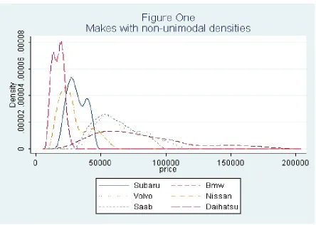
makes, as shown in Figure One, are broadly hump-shaped. With the exception of Daihatsu,
each has a tendency to have more flavors at high prices which is consistent with our model.
Calculation of the coefficient of skewness for each density reveals that nearly all of them
are positively skewed. For the seventeen makes, only one make had negative skewness (-0.32),
seven more had skewness statistics between 0.08 and 0.45, six more had skewness statistics
between 0.5 and 0.9 and three had skewness statistics between 1.82 and 3.52.
The final step we took to determine the typical shape of the densities of flavors was
14We use the GAUSS code of Henderson et al (2008) who applied the Cheng and Hall (1998) version of
to estimate a beta density function for each set of flavors.15 The beta density function is
described by two parameters,α andβ which can take on a wide variety of shapes depending
on their values. Before estimating the densities for each make, we had to transform the
data. This is because price is a continuous variable with similar cars selling for similar but
not identical prices. We obtained data for estimating the density function in three steps. In
the first step we construct a kernel estimate of the density for each make. Second, we select
values of the density function at 50 points. To ease estimation, we convert these values to
integers by multiplying them by 10 million and rounding. Descriptive statistics of the new
densities revealed they were similar to the descriptive statistics for the prices. However, we
will not be able to perform meaningful hypothesis tests with this new data.
If both parameters have values greater than one, then the distribution is unimodal and
hump-shaped. We find this to be the case for thirteen out of the seventeen makes. For one
make, BMW, α= 1 and β >1 which implies the density declines towards 0. The densities
of the other three brands are also downward sloping but in a J-shape. These makes tend
to be more expensive, including Audi and Saab. However, other premium makes, such as
Mercedes Benz and Volvo, were included among the thirteen.
Cheng and Hall (1998) suggest their calibration of the dip test may not be suitable for
highly skewed data and, from the results of estimating beta densities, three out of the four
makes with non-hump shaped distributions featured highly skewed distributions. Hence, for
robustness, we decided to re-perform the tests without the skewing observations. For the
nine makes with skewness coefficients of 0.5 or more, we dropped the top 10% of observations.
For the five makes with lower skewness after this, we performed the dip-test and re-estimated
the beta density functions to determine the influence of skewness on the results. For the dip
test, none of the makes we estimated were amongst those for which unimodality had been
rejected. The p-values on the test statistic fell for all of them, though not enough to change
the result. The results from estimating the beta density function were more striking. One of
the five had previously returned coefficients suggesting a J-shape. Now both α and β were
above one, and for the other four makes, their coefficients were much closer together. So it
seems as though skewness did not affect the dip statistic but it did affect the results from
estimating the beta density function.
The results from both a non-parametric test and estimating a density function are
consis-tent with the firms offering a hump shaped distribution of flavors. However, this descriptive
analysis doesn’t determine whether the pattern results from a strategy of flavor
prolifera-tion or is due to another cause. Before doing this, though, we need to explore alternative
explanations of the set of flavors offered by firms.
7.3
Alternative hypothesis
The primary alternative explanation of the pattern described in Section two is that firms
offer varieties if sufficient numbers of consumers demand each variety so to make it’s provision
profitable. In other words, the consumers differ substantially not only in their preferences
for quality, but also in their preferences for flavor, i.e. λ is sufficiently large.
Draganska, Mazzeo and Seim (2009) (hereafter DMS) provide a model of competition
by duopolists who choose price and which flavors of a product to offer that is designed for
estimation. Like the few other models for estimation that endogenize quality choices, the
set of flavors to be offered is chosen in the first stage of a two stage game. In the second
stage, given the set of flavors chosen by each firm, an equilibrium set of prices is chosen for
each set of flavors and consumers choose which products they purchase. Hence, the set of
flavors each firm chooses to offer is determined by the expected profitability of each flavor
in equilibrium.
DMS begin by modelling the second stage of competition given a set of flavors. On the
demand side DMS’s model obtains a flavor level demand equation by aggregating across
discrete choices of flavors by consumers, as developed by Berry et al. (1995). Denotesbf be
the market share of flavor f of brand (or firm) b which is a function of the flavor’s price,
and market demographics, ν:
sf b=f(pf b, p−f b, xf b, x−f b, ν) (49)
Total sales will equal the product of the market share and market size. On the supply
side, DMS assume firms engage in Bertrand competition with differentiated products. The
set of flavors offered for each brand can be represented by a vector of dummy variables, db,
where each element takes a value 1 if a flavor is offered. Each firm chooses a set of prices
to maximize profits from offering all of its flavors. Denote d−b as the set of flavors offered
by all of the other firms. The equilibrium set of prices offered by each firm are written as
a function of marginal cost, cbf and a markup term. All variable without subscripts denote
the set of variables offered by all firms:
pbf(db, d−b) = cbf +M Ubf(X, p, d, c, ν) (50)
Next DMS consider’s the first stage of competition. In this stage each firm chooses db to
maximize expected profits. Denote hb as the vector of fixed costs of firm b operating each
flavor and ¯Π(db) as the expected variable profit from offering db. The expected profit from
offering db is given by:
E[Πb(db, d−b] = ¯Π(db)−h′bdb (51)
Hence, the number of flavors offered by a firm at quality level, l, is modeled as:
nlb =f(X, h, c, ν, dlb) (52)
Production and entry costs are typically estimated rather than observable in most
econo-metric models of competition between differentiated products. The car industry is a lot more
complicated than the market analyzed by DMS, so it is not feasible to get estimates of these
by estimating a model like DMS’s. Furthermore, data on demographics specific to
between the number of flavors offered by a firm and all other flavors offered is not
straight-forward. Hence, it is infeasible to estimate even a reduced form model to test whether flavor
proliferation rather than demand and supply side factors determine the pattern of varieties.
Furthermore, there may be multiple sets of specifications of preferences and costs that
could generate a positive or hump shaped relationship between quality and variety. For
example, the variety of preferences could increase with income thereby supporting more
high quality variants in equilibrium. Alternatively, a hump-shaped distribution of varieties
could occur if a firm has low marginal costs (or low fixed costs) of producing a certain quality
level but higher costs for producing at any other level of quality. So using dummy variables
to control for many unobservable is unlikely to be successful. This model does not produce
a clear cut conclusion for the variety of flavors. In principle, one may expect distributions
of different modalities for different markets. The fact that the shape of the distribution is
similar across makes provides an indirect support for our theory.
7.4
A test of the hypothesis
The analysis of the previous subsection suggests determining if firms are engaging in
flavor proliferation by a reduced form analysis of the number of varieties by quality level by
make is unlikely to be feasible or successful. Instead, we propose a test of an implication of
our model that can be tested without relying on detailed controls for the determinants of
numbers of variants across distinct quality levels and segments of the market.
Specifically, whether the number of flavors offered by a firm increases with quality or
whether the number of flavors has a hump shaped relationship with quality, in both cases,
we expect a greater share of flavors offered by a firm to be associated with higher quality
models. While such a relationship could occur as a result of costs and preferences, our
analysis in Section 2 suggests this is unlikely.
We construct the test as follows. First, for each firm, we rank all varieties by price. The
null hypothesis is that the distribution of varieties over price, denoted n(p), is determined
all firms at that price, denoted S(p), is a good proxy. Sales are likely to be low for high
quality prestige cars because their development and production costs are so high as to enable
them only to be offered, in equilibrium, at a high price. The mark-up may be high but total
profits are unlikely to be too large. Sales are likely to also be low for very low quality small
cars because, in part, they have relatively poor characteristics and options and they face
competition from second hand higher quality cars. Though low quality cars can be produced
at a low cost and sold at a low price total profitability is unlikely to be high.
Hence, under the null hypothesis, the distribution of flavors at each price will not be
significantly different from the distribution of total demand at each price.
However, if our model is correct, then the distribution of sales should be to the left of the
distribution of flavors. At low quality levels, there will be relatively less flavors, compared
with demand, whereas at high quality levels there will be relatively more flavors compared
with demand. Formally:
FS(p)(z)≥Fn(p)(z) (53)
We specify ≥ for, as the distributions are compiled over the same range of prices, they
must ultimately meet.
To carry out this test, we perform two one-sided Kolmogorov-Smirnov tests of the equality
of distributions. Under the null hypothesis, the two distributions are identical. In the first
test, we test against the alternative that:
FS(p)(z)≥Fn(p)(z) (54)
In the second test, we test against the alternative that:
FS(p)(z)≤Fn(p)(z) (55)
If we reject the null hypothesis in the first test and fail to reject in the second, we
range of quality levels. Note, two tests are required for as the Kolmogorov-Smirnov test
selects points along the distribution it is possible that the distributions may cross and one
distribution may be significantly greater than and less than the other at different prices.
It is worth noting two measurement issues. First, we do not observe sales by variety but
by models or even groups of models. We estimate sales by variety by assuming each variety
has an equal share of the sales for the model. This may underestimate (and is unlikely to
systematically overestimate) sales for cheaper varieties within a model, which biases against
finding support for our model.
Second, as noted earlier, by not including sales of second hand cars, we are
under-estimating the sales of cars at, particularly, lower prices. Hence, we may find it harder to
reject the null hypothesis that the distribution of flavors matches that of sales at lower prices.
7.4.1 Test results
The test results are summarized in Table 3. In this table we report, with the makes
ordered by their mean price, the test statistics for the two Kolmogorov-Smirnov tests. First,
we note that the distribution of flavors is significantly below that of sales for all makes
except for Mazda, Toyota and the three cheapest brands. Furthermore, for all makes which
satisfy the first test, the distribution of flavors is never significantly above the distribution
of sales. Figures Two and three present the densities and distributions of sales and flavors
for the highest and lowest brands in this group - Subaru and Mercedes Benz. For Mercedes
Benz the two densities in the top panel demonstrate that the mass of varieties are provided
well to the right of mass of total sales across the range of prices at which Mercedes Benz
offers flavors. This leads to starkly different distribution functions in the lower panel. For
Subaru, which offers flavors priced below $50,000, while the distribution of flavors tracks
the distribution of sales at most prices, nevertheless at the higher prices, the distribution of
varieties is significantly below before rising rapidly at the very highest prices (quality levels).
Hence, most makes feature a distribution of flavors consistent with our model.
Mercedes-Benz and BMW suggests that this pattern is strategic rather than determined by
cost or preferences specific to particular segments of the market (like the variety of
prefer-ences increases with income).
It is also striking that the makes for which the three makes for which the model is not
supported are in the range where the measurement problems with sales are likely to be most
acute. Furthermore the densities of flavors offered by these makes are broadly similar to
those offered by the other makes. The results of the tests in subsection two reveal Hyundai
to have a hump shaped unimodal density of flavors. Figure One demonstrates Daihatsu and
Nissan have hump shaped (if not unimodal) densities.
8
Conclusions
In this paper we have analyzed theoretically and empirically the links between quality
and variety. The theoretical model has two components. First, consumers are modeled
as caring about quality but indifferent between varieties of the same quality. However, we
adapt a standard probabilistic choice model to introduce a very small amount of randomness
into consumer behaviour. The second component is a monopolist who engages in second
degree price discrimination. Faced with consumers which randomize, the profitability of price
discrimination is increased by the monopolist offering more varieties at higher qualities as
the likelihood that consumers choose high price products increases. If, at high quality levels,
the markets become sufficiently thin, though, the profit maximizing number of varieties falls,
yielding a hump-shaped relationship between variety and quality.
We then test these predictions using data on the product offerings of seventeen major
car companies in the Australian market. First, we demonstrate that most companies offer
a density of varieties that is hump shaped with respect to our proxy for quality, price. This
is a previously unidentified empirical regularity. We then determine that this distribution
is more likely to be due to flavor proliferation than just meeting demand for different
different from the distribution of varieties suggested by consumer demand. Another
impor-tant contribution of the paper is that the number of varieties offered by the market can be
higher than the social optimum even in the case of a single monopoly, which is opposite to
the conclusions drawn from the previous literature (see, Lancaster (1990)).
References
Anderson, S.P., dePalma, A. and Thisse, J.-F. Discrete choice theory of product
differentia-tion, MIT Press, Cambridge, MA, (1992).
Ansari, A., Economides, N. and Steckel, J. The max-min-min principal of product
differen-tiation, Journal of Regional Science, 38, 207-230, (1998).
Basov, S. Multidimensional Screening, Series: Studies in Economic Theory, volume 22,
Springer-Verlag: Berlin, (2005).
Basov, S. Monopolistic screening with boundedly rational consumers, The Economic Record,
85(S1), S29-S33, (2009).
Berry, S., J. Levinsohn and A. Pakes. Automobile Prices in Market Equilibrium.
Economet-rica, 63(4), 841 - 890, (1995).
Champsaur, P. and Rochet, J.-C. Multiproduct duopolists, Econometrica, 57(3), 533-557,
(1989).
Cheng, M.-Y. and Hall, P. Calibrating the excess mass and dip tests of modality, Journal of
the Royal Statistical Society, Series B, 60, 579-589.
Draganska, M. and Jain, D. C. Product-Line length as a competitive tool, Journal of
Eco-nomics and Management Strategy, 14, 1-28, (2005).
Draganska, M. and Jain, D. C. Consumer Preferences and Product-Line Pricing Strategies:
Draganska, M., M. Mazzeo and K. Seim, Beyond plain vanilla: Modeling joint product
assortment and pricing decisions, Quantitative Marketing and Economics, 7, 105-146,
(2009).
Glass’s Guide. Black and White Data Book, Glass’s Guide, Melbourne, (1998).
Henderson, D. J., Parmeter C. J., and R. R. Russell. Modes, weighted modes, and calibrated
modes: evidence of clustering using modality tests. Journal of Applied Econometrics,
23, 607-638, (2008).
Lancaster, K. The economics of product variety: A survey, Marketing Science, 9, 189-206,
(1990).
Luce R. D. Individual choice behavior, Wiley, New York, (1959).
Mas-Colell, A., Whinston, M. D. and Green, J. R. Microeconomic theory, Oxford University
Press, (1995).
Mussa, M. and S. Rosen. Monopoly and Product Quality, Journal of Economic Theory, 18,
310-317, (1978).
Neven, D. and Thisse, J. On quality and variety in competition, in Gabszewicz, J., Richard,
J. and Wolsley, J., (eds): Economic Decision-Making: Games, Econometrics, and
Opti-mization, Elsevier, Amsterdam, (1990).
Prentice, D. and Yin, X. Constructing a quality-adjusted price index for a heterogeneous
oligopoly, The Manchester School, 72, 423-442, (2005).
Shugan, S.M. Product assortment in triopoly, Management Science, 35, 304-320, (1989).
Stole, L. Lectures on contracts and organizations, (2000),
Table 1
VARIETIES OF NEW CARS IN AUSTRALIA, 1998 Category Features Price Reg’ns Makes Models Varieties
All 11 59.6 584.3 37 175 1081
Small 7 22.6 251.4 19 39 397
Medium 11 34.6 268.6 9 16 207
Luxury 15 114.3 47.9 26 97 390
Registrations per Models Varieties Category Make Model Obs. Per Make Per Make
All 15.79 3.33 0.54 4.73 29.22
Small 13.23 6.44 0.63 2.05 20.89
Medium 29.84 16.78 1.30 1.78 23.00
Luxury 1.84 0.49 0.12 3.73 15
Note: Price and Features data supplied by Glass’s Guide. Registrations data from Glass’s Guide (1998). Registrations is in thousands. Price is in thousand Australian dollars. All includes Small, Medium, Luxury, Sports and People Movers. Small combines the Glass categories of Small and Light. Medium combines the Glass categories of Medium and Upper Medium. Luxury combines the Glass categories of Prestige and Luxury. All cars are grouped by Glass Classification of the Model, or Make if no model detail.
Table 2
VARIETY PROLIFERATION AND VERTICAL DIFFERENTIATION BY FIRMS Ratio of Prices Number of Varieties Cases
Features per
Registration
Medium to Small 1.46 1.69 1.21 9
Luxury to Medium 1.72 1.42 5.13 3
Luxury to Small 2.04 1.56 1.89 5
(no Medium)
Each cell in the first three columns is calculated in three steps:
1. Calculate the average across varieties within each class for each firm 2. Take the ratio of the average across classes for each firm
3. Calculate the average ratio across firms
[image:34.612.79.557.379.488.2]Table 3
COMPARISON OF DISTRIBUTIONS OF SALES AND FLAVORS
Brand Tests
F(n((p))< F(S(p)) F(n(p))> F(S(p))
Daihatsu -0.0319 0.3116∗∗∗
Daewoo -0.1151 0.1372
Hyundai -0.0184 0.2781∗∗∗
Nissan -0.0554 0.4035∗∗∗
Toyota -0.078 0.075
Subaru -0.1507∗∗ 0.0193
Mazda -0.1041 0.0793
Mitsubishi -0.1579∗ 0.0991
Ford -0.1778∗∗∗ 0.0166
GM-Holden -0.219∗∗∗ 0.0046
Honda -0.3292∗∗∗ 0.0614
Volkswagen -0.3620∗∗∗ 0.0295
Saab -0.4773∗∗∗ 0.0278
Volvo -0.4370∗∗∗ 0.0222
Audi -0.574∗∗∗ 0.0263
BMW -0.5684∗∗∗ 0.0174
Mercedes Benz -0.7598∗∗∗ 0.0163
Appendix
In this Appendix, we draw on Anderson et al (1992) and Fudenberg and Levine (1998)
to compare four models of probabilistic choice. This comparison demonstrates two points.
First, under some reasonable assumptions, one can move freely between different
interpre-tations of random choice models. Second, that the Markovian and Machina-type models
provide an easier framework than the random-utility and address models, to analyse the
effect of introducing new varieties. Hence in the body of the paper we use the Luce model of
probabilistic choice as a particularly simple foundation for our model of consumer behavior.
Though one could use a random-utility or address model, modelling would just be more
complex.
Markovian learning models
Though these models originated in mathematical psychology in the work of Bush and
Mosteller (1955), they have been widely used in economics (e.g. Foster and Young (1990),
Fudenberg and Harris (1992), Kandori, Mailath, Rob (1993), Young (1993), Friedman and
Yellin (1997), Anderson, Goeree, and Holt (2004), Friedman (2000), and Basov (2003)).
Though most economic applications assume a continuous choice space, for simplicity of
presentation and for consistency with our application, we assume a finite choice space.
Suppose an individual faces a choice among n different options. A boundedly rational
individual is assumed to start with a random choice and adjust her choice over time in a way
that appears beneficial given her current experience. From time to time the individual may
also experiment. This kind of behavior usually leads to a Markov process over the choice
space, which can be described as:
pt+1 =f(pt, u), (56)
wherepτ ∈∆n is the vector of choice probabilities at timeτ , u∈Rn is the vector of utilities
associated with different choices, f : ∆n → ∆n is a continuous function and ∆n is the n−