Munich Personal RePEc Archive
Locational signaling and agglomeration
Berliant, Marcus and Yu, Chia-Ming
Washington University in St. Louis
19 December 2009
Locational Signaling and Agglomeration
∗
Marcus Berliant
†and Chia-Ming Yu
‡December 19, 2009
Abstract: Agglomeration can be caused by asymmetric information and a locational signaling effect: The location choice of workers signals their pro-ductivity to potential employers. The cost of a signal is the cost of housing at a location. When workers’ price elasticity of demand for housing is negatively correlated with their productivity, skill-biased technological change causes a core-periphery bifurcation where the agglomeration of high-skill workers eventually constitutes a unique stable equilibrium. When workers’ price elas-ticity of demand for housing and their productivity are positively correlated, skill-biased technological improvements will never result in a core-periphery equilibrium. This paper claims that location can at best be an approximate rather than a precise sieve for high-skill workers. (JEL Classifications: D51; D82; R13)
Keywords: Agglomeration; Adverse Selection; Asymmetric Information; Locational Signaling
∗We thank Karl Dunz, Yasuhiro Sato, participants at the 2009 North American Meet-ings of the Regional Science Association International, and participants at the spring 2009 Midwest Economic Theory meetings for comments. The second author acknowledges fi-nancial support from the Center for Research in Economics and Strategy (CRES) at the Olin Business School, Washington University in St. Louis. The authors retain responsi-bility for the contents of this paper.
†Department of Economics, Washington University, Campus Box 1208, 1 Brookings Drive, St. Louis, MO 63130-4899. Phone: (1-314) 935-8486, Fax: (1-314) 935-4156, e-mail: [email protected]; and Division of the Humanities and Social Sciences, California Institute of Technology.
1
Introduction
As shown in Baum-Snow and Pavan [2009], US wages were more than 30
percent higher in metropolitan areas with over 1.5 million inhabitants than
in rural areas in the year 2000. Furthermore, their model indicates that
abil-ity sorting and returns to experience across locations are crucial elements in
explaining the wage premium in large cities. Glaeser and Mare [2001] show
that sorting on human capital accounts for about one-third of the city-size
wage gap in the US. Moreover, Gould [2007] demonstrates that migration
of high-skill workers is important in justifying the urban productivity
pre-mium which is amplified by steeper experience profiles in urban areas. These
analyses suggest that workers signal their skill and experience using their
locations. That is, the location choice of workers can signal their
produc-tivity to potential employers. The signaling cost is the price of housing at
a location. Locational signaling is also consistent with a constant product
of city rankings and growth rates in population for top-ranking cities: The
U.S. Census Bureau data show that, from 1990 to 2000, this constant is
around 0.11 for the top three cities.1
That is, though housing rents are high
and population is dense in top-ranking cities, these costs do not inhibit new
migrants from moving in. This paper analyzes the effects of locational
sig-naling behavior, in particular how and whether locational sigsig-naling effects
can generate agglomeration.
One natural question is: How can we empirically distinguish locational
signaling effects from agglomeration externalities? Agglomeration
external-ities and spillovers are widely analyzed in the literature, for example,
Hen-derson [1986], HenHen-derson et al. [1995], Glaeser et al. [1992], and Feldman
and Audretsch [1999]. Under the framework of agglomeration externalities,
1
an increase in the ratio of high-skill labor in one region causes more than a
proportional increase in the average real wage (or an increase in labor’s
mar-ginal product). In a locational signaling model, an increase in the ratio of
high-skill labor in a region yields a proportional increase in the average real
wage. The predictions of a signaling model are consistent with the findings
in Aghion et al. [1999, p. 1644]: “The main argument put forward against
the skill-biased technical change hypothesis is that we have not observed an
increase in the rate of productivity growth since the early 1980s.”
Households’ private information includes their productivity, which varies
among individuals. When locations can possibly reveal workers’
productiv-ities, it is natural to ask why in practice some locations are attached to a
signal for high productivity of workers, while others are not. For example,
fashion designers in Milan, software programmers in Seattle, entertainers in
Hollywood, financiers on Wall Street, or high-tech workers in Silicon Valley
can be viewed as having a higher productivity than do workers in the same
field in other locations. These observations could be due to learning from
other workers, or interaction with R&D in these locations; however, they
could also due to a locational signaling effect. Many tools are used to signal
workers’ abilities since information about workers’ skill is very important to
firms and workers, for example: college diplomas, professional certificates,
and academic alliance memberships.2
It is interesting to examine how
high-skill workers can use locational agglomeration to distinguish themselves from
other workers, and how effective location can be as a reference for workers’
productivity.
In the literature, Starrett [1978] proves a spatial impossibility theorem:
If there is no relocation cost, space is homogeneous (consumers’ preferences
and firms’ technologies are independent of location), the economy is closed,
and there are perfect and complete markets everywhere, there is no
compet-2
itive equilibrium involving costly transportation of any commodity. Fujita
and Thisse [2002] interpret this theorem further and show that either there
is no agglomeration of agents in equilibrium or there is no equilibrium at all.
However, Starrett’s theorem offers only sufficient conditions for no
agglom-eration in equilibrium; these conditions are not necessary. Therefore, when
one of the conditions is violated, it is not clear whether firms or workers will
agglomerate or not. Berliant and Kung [2008] is the first paper analyzing
how asymmetric information causes agglomeration. Using a screening model,
they show that workers can agglomerate and be sorted by skill in equilibrium
due to asymmetric information in the labor market. This paper focuses on
a complementary question: When there is asymmetric information, does an
agglomeration emerge in equilibrium due to the signaling value of the choice
of location? The shadow cost of location, and thus of the signal, is the price
of housing in the region.
Krugman [1991a] and New Economic Geography models adopt increasing
returns to scale to explain the agglomeration of manufacturing firms in one
region. When transportation cost is decreased as transportation technology
is improved, a core-periphery pattern is more likely in equilibrium. It is
natural to ask: Is a core-periphery configuration more likely to constitute an
equilibrium when there are no increasing returns to scale in production, but
rather asymmetric information?
Many economic agglomeration phenomena in reality cannot be
satisfac-torily explained by increasing returns to scale. As expounded in Krugman
[2009], “the history of such classic localizations as that of the car industry
seemed to suggest that concentrations due to increasing returns peaked
be-fore World War II.” Thus, ”there is good reason to believe that the world
economy has, over time, actually become less characterized by the kinds
of increasing-returns effects emphasized by new trade and new geography.”
increas-ing returns to scale in explainincreas-ing the agglomeration of industries without
increasing returns. A signaling incentive potentially fills this need.
In contrast to considering aggregate uncertainty in Berliant and Yu [2009],
idiosyncratic uncertainty (individual specific information) is the source of
asymmetric information in this paper. We consider a model with two
homo-geneous regions and two types of workers, with high and low productivity,
respectively. Workers are mobile across regions while differences in regional
wages and housing rents determine their migration incentives. We first
an-alyze the case when workers’ price elasticity of demand for housing is
neg-atively correlated with their productivity. In this case, as shown in Figure
10, there are at least three equilibria: a completely symmetric equilibrium
where every type of worker is evenly distributed over both regions, and two
partially segregated equilibria (or say core-periphery equilibria) where
high-productivity workers are agglomerated in one region. The partially
segre-gated equilibria are always stable. When the difference in workers’
produc-tivities is small, the completely symmetric equilibrium is stable; when the
difference in workers’ productivity is large enough, the completely symmetric
equilibrium becomes unstable. When the difference in workers’ productivity
is very large, in addition to the unstable completely symmetric equilibrium
and two stable core-periphery equilibria, there are two unstable
asymmetri-cally integrated equilibria. On the other hand, when workers’ price elasticity
of demand for housing is positively correlated with workers’ productivity, as
shown in Figure 9, there always exists a completely symmetric equilibrium
but there is no core-periphery equilibrium. The completely symmetric
equi-librium is stable when the difference in workers’ productivities is not large.
When the difference in productivities is very large, there are three unstable
equilibria where one of them is completely symmetric and two of them are
asymmetrically integrated equilibria.
indus-try in Milan attracts workers in an alternative region to migrate to Milan,
due to a larger aggregate housing demand, there will be a higher housing
rent in Milan to offset workers’ migration incentives. As shown in Figure
1,3
when high-productivity workers have a lower price elasticity of demand
for housing than low-productivity workers, the utility cost of signaling for
high-productivity workers is lower than the utility cost of signaling for
low-productivity workers at the core-periphery equilibrium. Therefore, for a
given wage premium in Milan, there is a long-run segregated equilibrium
such that all the high-productivity workers agglomerate in Milan while the
low-productivity workers reside in both Milan and the alternative region.
When high-productivity workers have a higher price elasticity of demand for
housing than low-productivity workers, as shown in Figure 2, the signaling
cost for high-productivity workers is higher than that for low-productivity
workers under any core-periphery configuration. This intuition is verified in
this paper, which suggests a potentially testable implication of our model,
namely the prevalence of agglomeration of high-skill workers as a function of
the correlation of skill and demand elasticity for housing.
Notice that, in either a segregated or an integrated equilibrium, no region
is fully occupied by high-productivity workers alone. That is, there is no
completely segregated equilibrium, but a semi-pooled equilibrium may exist.4
On the other hand, there is always a completely pooled equilibrium in our
model. Therefore, it is only possible to ensure that any worker who does not
reside in Milan is a low-productivity worker. For every worker in Milan, it is
impossible to guarantee that his/her productivity is high in any equilibrium.
This observation indicates that location at best is an approximate instead of
a precise sieve for high-productivity workers.
3
We shall explain the figures introduced here in detail later in the paper. This is a preview.
4
Furthermore, if we consider a continuous increase in high-skill workers’
productivity relative to that of low-skill workers, a core-periphery fork
bifur-cation is present (Figure 10), even if there are no increasing returns to scale
in production and knowledge spillovers. In other words, the agglomeration of
high-productivity industries can be attributed to the existence of a locational
signaling effect. Since, intuitively, increasing returns to scale in fashion
de-sign seems bizarre, the agglomeration of fashion industries in Milan can be
explained from a signaling viewpoint.
Signaling cost in our model is determined by housing prices, and housing
prices are different for different distributions of workers. In contrast with
most signaling models where the marginal signaling cost is exogenous, i.e.,
Spence [1973], Wilson [1977], Grossman [1981], and Rothschild and Stiglitz
[1976], the marginal signaling cost is endogenous in our paper. That is,
signaling cost affects workers’ migration incentives, and after their migration,
the distribution of workers’ types further influences the signaling cost. We
explore the question: Does the interaction between migration and marginal
signaling cost yield a separated equilibrium? The same type of endogeneity
also holds in cheap-talk models like Crawford and Sobel [1982] and
Austen-Smith and Banks [2000].
In what follows, our model is introduced in Section 2. Additionally,
nec-essary and sufficient conditions for the existence of stable core-periphery
equilibria and for the stability of integrated equilibria are presented.
Sev-eral numerical examples and related welfare analyses are offered in Section
3. Conclusions are in Section 4.
2
Model
There are two regions k ∈ K ≡ {x, y} with the same land endowment ¯s.
nH, nL ∈
R++, respectively, where the productivity of H-type workers is
higher than that of L-type workers. H-type (L-type) workers can be
in-terpreted as high-skill (low-skill) workers, or can be inin-terpreted as
experi-enced (novice) workers. With the second interpretation, the appearance of
a segregated equilibrium implies that returns to experience are important in
explaining city size wage premium.
Throughout this paper, workers’ type is indexed by a superscript and
location is indexed by a subscript. The (endogenous) population of i-type
workers living in k is denoted by ni
k, and the (exogenous) aggregate
popula-tion in the model isn =nH+nL. Firms cannot recognize any worker’s type
directly; however, firms know the (equilibrium) distribution of workers’ types
over the two regions and can infer the probability of a worker’s type using
his/her location. Utility is CES. Let si
k, zik be each i-type worker’s house
size and the consumption of composite goods in region k, i ∈ N, k ∈ K,
respectively. Let pk denote the rent per unit of housing and wk denote the
worker’s wage in k, k ∈ K. Each worker is endowed with one unit of labor.
The rents are collected and consumed by an absentee landlord, denoted byA,
who is endowed with all the housing. Letϕi k≡(s
i k, z
i
k),i∈N∪ {A},k ∈K.
The absentee landlord has an inelastic supply of housing ¯s in each region
and maximizes the rent that he can collect, i.e., maxzA k
P k∈Kz
A
k, subject to
zA
k ≤pks,¯ ∀k ∈K, and has an inelastic supply of housing in all cities.5 The
optimization problem for H-type workers in regionk, k ∈K, is
max uH
k(ϕHk ) = [(sHk) α−1
α + (zH k )
α−1 α ]
α α−1
s.t. pksHk +z H
k ≤wk, (1)
sHk, z H
k ∈R+; 5
whereas the optimization problem for L-type workers in k is
max uLk(ϕ L k) = [(s
L k)
β−1 β + (zL
k) β−1
β ] β β−1
s.t. pksLk +zkL≤wk, (2)
sL k, z
L
k ∈R+.
Assume thatα, β >1. Eitherα > β holds, which implies that workers’ price
elasticity of demand for housing is positively correlated with productivity, or
α < β holds, implying that workers’ price elasticity of demand for housing
and productivity are negatively correlated.6
To simplify the analysis, assume that each worker inelastically supplies
one unit of labor, so we need not be concerned about monitoring and
vol-untary participation constraints. Every firm hires one worker at most. Each
firm can adopt a high type technology together with a H-type labor to
pro-duce YH, or adopt a low type technology together with a L-type labor to
produce YL, where 0 < YL < YH. The corresponding profit in k is YH−w k
and YL−w
k, respectively, k ∈K. When any firm adopts a high type
tech-nology with a L-type worker, the output is zero. On the other hand, when a
firm adopts a low type technology and a H-type worker, the output is YL,
which is lower than YH. That is, no firm would prefer to adopt a technology
that is incompatible with the type of the hired worker. Firms maximize their
expected profit, and their actual behavior in choosing technology will be
ex-plained later. Every firm or worker is so small that he/she cannot influence
competitive market prices. Furthermore, assume that there is free entry of
firms, and thus, every firm earns zero expected profit in equilibrium. Finally,
workers choose locations to maximize their utilities, including the
considera-tion that firms can possibly learn about workers’ types only from observing
their locations.
6
To extract the influence of signaling effects, assume that there is no
com-muting; that is, workers can work only in the place where they live. In other
words, this is a regional, not city, model. However, H-type andL-type
work-ers are allowed to migrate to earn a higher utility.7
Denote ρH (ρL) as the
ratio of H-type (L-type) workers in the world living in x, and thus 1−ρH
(1−ρL) is the ratio of all H-type (L-type) workers living in y. The
popula-tion in x and y, given (ρH, ρL), can be expressed as n
x =ρHnH +ρLnL and
ny = (1−ρH)nH + (1−ρL)nL, respectively.
To characterize locational signaling effects, the market process is given as
follows. First, each firm hires a worker without knowing his/her productivity.
Though firms do not know each worker’s type, suppose that firms do not
misperceive; that is, they know the actual equilibrium proportion of H-type
workers in each region and thus have a common distribution over a worker’s
type conditional on his/her equilibrium location. Then, since there is a free
entry of firms, each firm in a region pays its worker a wage according to the
expected profit in the region. After learning the type of worker that the firm
hires, the firm chooses its production technology to maximize ex post profit
or minimize ex post loss. A mixed adoption of technology is assumed not
available for firms.8
Note that given (ρH, ρL), since there is free entry of firms, each firm earns
7
WhenH-type workers are mobile butL-type workers are immobile, there are similar bifurcations.
8
zero expected profit. Thus, the wages for every worker in regionxandy are9
wx(ρH, ρL) =
1 nx
(ρHnHYH +ρLnLYL), (3)
wy(ρH, ρL) =
1 ny
[(1−ρH)nHYH + (1−ρL)nLYL]. (4)
Let us temporarily leave workers’ mobility aside. Short-run equilibrium is
defined as a competitive market equilibrium, given a population distribution
over the two regions.
Definition 1 (Short-Run Equilibrium)
(ϕH∗ k , ϕL
∗ k , ϕA
∗ k , w
∗ k, p
∗
k)k∈K constitutes a short-run equilibrium if, given an
ar-bitrary (ρH, ρL), workers choose optimal consumptions, firms make
compet-itive wage offers for the distribution of workers, and the housing and the composite good markets in each region clear. That is:
(a) ui k(ϕi
∗
k)≥uik(ϕik), for allϕik ∈R
2
+ satisfying pksik+zki ≤wk, ∀i∈N,
k ∈K; (b) w∗
x=
1
nx(ρ H∗
nHYH +ρL∗
nLYL), and
w∗ y =
1
ny[(1−ρ H∗
)nHYH + (1−ρL∗
)nLYL];
(c) ρH∗
nHsH∗ x +ρL
∗
nLsL∗ x = ¯s,
(1−ρH∗
)nHsH∗
y + (1−ρL ∗
)nLsL∗ y = ¯s,
(ρH∗
zH∗
x + (1−ρH ∗
)zH∗
y )nH + (ρL ∗
zL∗
x + (1−ρL ∗
)zL∗
y )nL+zA ∗ x +zA
∗ y
=nHYH +nLYL, where zA∗
k =pk¯s, k∈K.10
The short-run equilibrium, by Walras’ law, is determined by conditions
(a), (b), and the first two (or the last two) equalities in (c). Theorem 1 shows
that the short-run equilibrium exists and is unique.
Theorem 1 For each(ρH, ρL)∈[0,1]×[0,1], there exists a unique short-run
equilibrium.
9
The main purpose of this paper is to characterize agglomeration across regions, instead of migration within one region; therefore, wage inequality within the same region is not considered here.
10
Proof. It is obvious from (b) that w∗
k = wk(ρH, ρL), k ∈ K, can not be
empty or multiple-valued. Substituting w∗
k into workers’ utility
maximiza-tion problems (1) and (2), we have workers’ optimal consumpmaximiza-tions as
func-tions of pk and (ρH, ρL); that is, ϕHk(pk, wk(ρH, ρL)) = [wk(ρH, ρL)/(pk +
pα
k), wk(ρH, ρL)/(1 +p
1−α
k )] and ϕLk(pk, wk(ρH, ρL)) = [wk(ρH, ρL)/(pk+pβk),
wk(ρH, ρL)/(1 +p
1−β
k )], all are well-defined demand functions. Finally, the
equilibrium housing prices can be solved from substituting demands into
market clearing conditions, i.e., ρHnH sH
x(px, wx∗) +ρLnLsLx(px, w∗x) = ¯s and
(1−ρH)nHsH
y (py, w∗y) + (1−ρL)nLsLy(py, wy∗) = ¯s. Though there are no
ex-plicit solutions for these two equalities, we can solve housing prices for each
given (ρH, ρL), and since the excess demand function for housing ink,k ∈K,
is continuous and monotonically decreasing inpx andpy, for allpx,py ∈R++,
p∗
k = pk(ρH, ρL) is uniquely determined for each (ρH, ρL). Accordingly, we
have well-defined equilibrium consumptions, ϕi∗
k =ϕik(p ∗ k, w
∗
k) = ϕik(ρH, ρL),
i∈N, k ∈K. Q.E.D.
When workers’ mobility is considered, workers have to choose their
opti-mal locations according to the utilities from living in the two regions. Since
i-type workers’ indirect utility from living in region k is ui k(ϕi
∗
k), i ∈ N,
k ∈K, the equilibrium condition for no further migration is
ui x(ϕ
i∗ x) =u
i y(ϕ
i∗
y ), if ρ i∗
∈(0,1), ∀i∈N. (5)
However, when all i-type workers are agglomerated in region k, i∈ N, k ∈
K, i-type workers’ utility in the other region k′, k′ ∈ K where k′ 6= k, is
not defined. Following the literature, the potential wage and housing rent
for i-type workers in k′
is defined as the limit of the equilibrium wage and
equilibrium rent in k′
when the ratio ofi-type workers ink′
approaches zero.
Then, the potential utility for i-type workers in k′
is defined according to
their potential wage and potential housing rent in k′
. Given this setting,
the signaling equilibrium concept is in fact defined by a pair (ρH∗
, ρL∗
[0,1]×[0,1], and the corresponding (ϕH∗ k , ϕ
L∗ k , ϕ
A∗ k , w
∗ k, p
∗
k)k∈K that satisfies
following conditions.
Definition 2 (Signaling Equilibrium)
((ϕH∗ k , ϕL
∗ k , ϕA
∗ k , w
∗ k, p
∗
k)k∈K, ρH∗, ρL∗)constitutes a signaling equilibrium when
(ϕH∗ k , ϕL
∗ k , ϕA
∗ k , w
∗ k, p
∗
k)k∈K constitutes a short-run equilibrium for (ρH∗, ρL∗),
and, in addition, no worker in any region has an incentive to migrate to the other region. That is, in addition to conditions (a)-(c) in Definition 1, it is required that
(d) ui x(ϕi
∗
x) =uiy(ϕi ∗ y) if ρi
∗ ∈(0,1), ∀i∈N, k ∈K;
uH x(ϕH
∗
x )≥limρH→1uHy (ϕHy [py(ρH, ρL∗), wy(ρH, ρL∗)]), if ρH∗ = 1;
uL x(ϕL
∗
x )≥limρL→1uLy(ϕLy[py(ρH∗, ρL), wy(ρH∗, ρL)]), if ρL∗ = 1;
uH y (ϕH
∗
y )≥limρH→0uHy (ϕHy [py(ρH, ρL∗), wy(ρH, ρL∗)]), if ρH∗ = 0;
uL y(ϕL
∗
y )≥limρL→0uLy(ϕLy[py(ρH∗, ρL), wy(ρH∗, ρL)]), if ρL∗ = 0.
The long-run signaling equilibrium can be solved by a system of equations
including (a), (b), (d), and, by Walras’ Law, the first two (or the last two)
equations of condition (c) in Definition 1. That is, the equilibrium housing
rents are determined by
hx ≡ρHnH(px+pαx) −1
+ρLnL(px+pβx) −1
− ¯s wx
= 0, (6)
hy ≡(1−ρH)nH(py+pαy) −1
+ (1−ρL)nL(p
y +pβy) −1
− s¯ wy
= 0. (7)
Substituting equilibrium consumption and equilibrium prices into the utility
functions, we have workers’ difference in indirect utilities from living in the
regions. Letting ui∗
k = uik(ϕi ∗
k), in order to have an easy decomposition of
utility functions.11
loguH∗
x −logu H∗ y
= (logwx−logwy)−
log(1 +p1−α x )
−1
α−1 −log(1 +p1−α y )
−1 α−1
, (8)
loguL∗
x −logu L∗ y
= (logwx−logwy)−
log(1 +p1−β x )
−1
β−1 −log(1 +p1−β y )
−1 β−1
. (9)
Notice that logwx−logwy is interpreted as a signaling gain (if it is positive),
or signaling loss (if it is negative) from living in x comparing to living in y,
which is the same for both types of workers. On the other hand, the signaling
cost of living inxrelative to living inyis log(1 +p1−α x )
−1
α−1 −log(1 +p1y−α) −1 α−1
and log(1 + p1−β x )
−1
β−1 − log(1 + p1−β y )
−1
β−1 for H-type and L-type workers,
respectively.
Equilibrium is a solution to a system of four nonlinear simultaneous
equa-tions (6), (7), (8), and (9). It is interesting to notice that if (ρH∗, ρL∗) = (1 2,
1 2)
constitutes an equilibrium, the result is exactly the case where both types
of workers are equally distributed over the two regions, which is called a
completely symmetric equilibrium; whereas if either (ρH∗
, ρL∗
) = (1,0) or
(ρH∗
, ρL∗
) = (0,1) in equilibrium, there is a segregated equilibrium. Letting
f ≡loguH∗
x −loguH ∗
y and g ≡loguL ∗
x −loguL ∗
y , the following lemma ensures
the existence of an interior equilibrium.
Lemma 1 Equal-dispersion(ρH∗
, ρL∗
) = (1/2,1/2) always constitutes a sig-naling equilibrium.
Proof. Given (ρH, ρL) = (1/2,1/2), it is known that w
x =wy, and from (6)
and (7), it can be checked that px =py. Since wx = wy and px = py imply
f = 0 and g = 0, we have that (ρH, ρL) = (1/2,1/2) is always one of the
solutions to (6), (7) and loguH∗
x = loguH ∗
y , loguL ∗
x = loguL ∗
y . Q.E.D.
In addition to the existence of a signaling equilibrium, the stability of a
11
Since YL >0 impliesw
x, wy >0, the CES indirect utilities are greater than 0, so it
long-run equilibrium should also be examined. The definition of stability for
an equilibrium is given as follows.
Definition 3 (Stability of Equilibrium)
For any small deviation of one type of workers from the equilibrium worker distribution, given that firms can only recognize a worker’s type according to their beliefs generated by the worker’s equilibrium location, if the utility difference from living in different locations drives the perturbed workers back to their equilibrium locations, the equilibrium is stable; otherwise, the equi-librium is called unstable.
Note that, given condition (d) in Definition 2, a core-periphery
config-uration (i.e, ρH∗
= 0 or ρH∗
= 1) is always a stable equilibrium when it
constitutes an equilibrium. However, a completely symmetric equilibrium
can be stable or unstable.
For a given (logui∗
x, logui ∗
y), i∈N, we consider standard dynamics with
multiple types of workers. When logui∗
x >logui ∗
y (logui ∗
x <logui ∗
y), i∈ N,
i-type workers in y (x) surely have incentive to move to x (y). In order
to explore the stability of signaling equilibria, following Krugman [1991b],
Fukao and Benabou [1993], and Forslid and Ottaviano [2003], for i ∈N, let
˙
ρi describe the ad hoc dynamics:
˙
ρi ≡ dρ i dt =
max{0, γ(logui∗
x −logui ∗
y)} if ρi = 0,
γ(logui∗
x −logui ∗
y ) if ρi ∈(0,1),
min{0, γ(logui∗
x −logui ∗
y )} if ρi = 1.
(10)
Notice that γ > 0 represents a measure of the speed of adjustment in the
ratio of i-type workers across regions, i ∈ N (as emphasized in Krugman
[1991b], “γ is an inverse index of the cost of adjustment”). That is, when
logui∗
x > logui ∗
y (logui ∗
x < logui ∗
y), i-type workers in y (x) migrate to x
(y) with a speed of |ρ˙i|. From the specified ad hoc dynamics, two curves
corresponding to ˙ρH = 0 and ˙ρL = 0 can be drawn on the (ρH, ρL) plane as
Intuitively, when ρH increases, fixing ρL and all parameters, since the
population inx(y) increases (decreases), the demand for and the equilibrium
price of houses inx(y) increase (decrease) and at the same time, the average
productivity or wage of workers in x (y) increases (decreases). Therefore,
logui∗
x −logui ∗
y ,i∈N, may not be a monotonic function ofρH. On the other
hand, given ρH and parameters, when ρL increases, the demand for housing
in x increases and the average productivity of workers in x decreases. That
is, there is no benefit but only damage for any resident in x when there are
low-skill migrants coming from y, so logui∗
x −logui ∗
y,i∈N, is monotonically
decreasing in ρL. Notice that the signaling gain is the same for both types
of workers in the same region. As illustrated in Figure 1, when the price
elasticity of demand for housing forH-type workers is smaller than that for
L-type workers, the signaling cost forH-type workers is less than the signaling
cost for L-type workers at the core-periphery equilibrium, and thus, H-type
workers have a stronger incentive to migrate to the region with a higher wage,
which causes an agglomeration of H-type workers in the ex post core region.
By contrast, in Figure 2, when the price elasticity of demand for housing for
H-type workers is larger than that forL-type workers, the signaling cost for
H-type workers is higher than the signaling cost for L-type workers. In this
case, there is no equilibrium with an agglomeration of any type of worker.
In the interesting cases with nH < nL, these intuitions are verified by the
following numerical simulations.
3
Numerical Examples
Since there is no closed-form solution for the simultaneous equations (6)-(9),
some numerical examples are analyzed here. Given nH = 1, nL = 2,YL = 1,
¯
s = 1,α= 2,β = 4, andYH = 1.25, a corresponding phase diagram is shown
negatively correlated. In the phase diagram, from f ≡ loguH∗
x −loguH ∗ y
and g ≡ loguL∗
x −loguL ∗
y , it can be checked that ˙ρH < 0 ( ˙ρH > 0) for all
(ρH, ρL)-points above (below) the curve of ˙ρH
= 0. In addition, ˙ρL < 0
( ˙ρL >0) for all (ρH, ρL)-points above (below) the curve of ˙ρL
= 0. Letting
φi(ρH) = {ρL|logui∗
x(ρH, ρL) = logui ∗
y (ρH, ρL)}, i ∈ N, the phase diagram
shows that φi(ρH), i ∈ N, is single valued and non-empty for ρH ∈ [0,1].
The phase diagram also shows that a necessary and sufficient condition for
a stable completely symmetric equilibrium is φH′(ρH) ≤ 0 at ρH = 1/2.
A sufficient condition for the existence of a core-periphery equilibrium is
φL(ρH)< φH
(ρH) atρH = 1 or φL
(ρH)> φH
(ρH) at ρH = 0. All these
con-ditions are satisfied in Figure 3 where there exist three equilibria: one stable
completely symmetric equilibrium and two stable core-periphery equilibria at
(ρH∗
, ρL∗
) = (0,0.61) and (ρH∗
, ρL∗
) = (1,0.39). At (ρH∗
, ρL∗
) = (1/2,1/2),
uH∗ x =uH
∗
y = 2.28,uL ∗ x =uL
∗
y = 1.44, and uA
∗ = 1.81. Since firms’ expected
profit is zero in all equilibria, ex ante social welfare function is defined as
the sum of workers’ and the landlord’s utilities. The social welfare equals
6.97 in the completely symmetric equilibrium, which is higher than the
so-cial welfare of 6.94 at any core-periphery equilibrium.12
The reason is that
locational signaling is unproductive, and thus it is not socially optimal to
agglomerate high-skill workers in our model.
Given the same parameters, when YH increases to 2, as shown in Figure
4, the completely symmetric equilibrium becomes unstable, though there are
still two stable core-periphery equilibria, (ρH∗
, ρL∗
) = (0,0.41) and (ρH∗
, ρL∗
) =
(1,0.59). WhenYH = 4, besides the two core-periphery equilibria at (ρH∗
, ρL∗
) =
(0,0.23) and (ρH∗
, ρL∗
) = (1,0.77), there are three unstable integrated
equi-libria at (ρH∗
, ρL∗
) = (0.09,0.27), (ρH∗
, ρL∗
) = (1/2,1/2), and (ρH∗
, ρL∗
) =
(0.91,0.73). In both the cases of YH = 2 and 4, ex ante social welfare in
12
Since at (ρH∗, ρL∗) = (1,0.39), uH∗
x = 2.27, uHy∗ = 2.25, uLx∗ = uLy∗ = 1.43, and
the completely symmetric equilibrium is higher than that in other
equilib-ria. Letting WCS, WAI, and WCP denote social welfare in the completely
symmetric, asymmetrically integrated, and coperiphery equilibrium,
re-spectively, it can be checked that WCS > WAI > WCP for all YH >2.
A core-periphery bifurcation is present when a high-skill biased
techno-logical improvement is considered as a continuous process. Denote YH(S)
as the sustain point where a given core-periphery pattern can be sustained,
i.e., YH(S) = min{YH|φH
(1) ≥ φL(1)}, and YH(B) to be a break point
where the symmetric equilibrium starts to become unstable, i.e., YH(B) =
{YH|φH′
(1
2) = 0}. As shown in Figure 10, given the above parameters and
when α= 2, β= 4, the sustain point is at YH(S) = 1 while the break point
is at YH(B) = 1.56. It can be checked that in all core-periphery
equilib-ria, population in the core region is larger than population in the periphery
region. Moreover, the difference in population of different regions increases
with the difference between YH and YL. The divergent trends in urban and
rural population are confirmed by data in U.S. Census Bureau [1990] (Table
1) which shows that in addition to the increasing difference in urban and
rural population, the percentage of US urban population in total
popula-tion is increasing over time, and the percentage of US rural populapopula-tion is
decreasing from 1950 to 1990.
On the other hand, when productivity and the elasticity of demand for
land are positively correlated, given nH = 1, nL = 2, YL = 1, ¯s = 1, α= 4,
β = 2, and YH = 1.25, the unique equilibrium is completely symmetric
which is also stable. When YH = 2, the unique completely symmetric
equi-librium is unstable. When YH further increases to be 4, there are three
integrated equilibria at (ρH∗
, ρL∗
) = (0.09,0.31), (ρH∗
, ρL∗
) = (1/2,1/2), and
(ρH∗
, ρL∗
) = (0.91,0.69). None of these integrated equilibria is stable and
there is no core-periphery equilibrium. Moreover, social welfare in the
As shown in Figure 9, whenα= 4, β = 2, the break point is atYH(B) =
1.78 and there is no core-periphery equilibrium for all YH > YL. Finally,
denote YH(F) as a bifurcation point where the number of interior equilibria
starts to be greater than 1. As shown in Figures 5 and 8, YH(F) is the YH
value such that when the relative positive steepness of curves with ˙ρH = 0 and
˙
ρL = 0 at (ρH, ρL) = (1/2,1/2) starts to switch, i.e.,YH(F) ={YH|φH′
(1 2) =
φL′(1
2)}, it can be checked thatY
H(F) = 2 for both cases withα= 2, β = 4,
and α= 4, β = 2. The dotted curves in Figures 10 and 9 represent unstable
equilibria and solid lines represent stable equilibria.
Beginning from a uniform distribution of both types of worker over the
two regions, when a skill-biased technological change is considered (that is,
YH increases over time while YL is a constant), when α < β, we can have
a core-periphery bifurcation as shown in Figure 10. As the productivity
of skill workers increases, since the signaling cost is lower for
high-skill workers than low-high-skill workers around (ρH, ρL) = (1/2,1/2), high-skill
workers have a stronger incentive to deviate to another region than low-skill
workers once the distribution of workers is slightly perturbed. The breakdown
of the uniform distribution of workers leads to a migration of some high-skill
workers from one region (ex postperiphery) to another region (ex postcore),
namely the “first migration wave.” After the migration of these high-skill
workers, firms start to notice the difference between average productivities in
the two regions, and thus, a positive signaling effect is attached to the region
with a higher ratio of high-skill workers. That is, firms start to pay workers
different wages according to their locations. Though short-run equilibrium
housing cost in the region with a higher ratio of high-skill workers increases
(and housing cost in the other region decreases), both high-skill and
low-skill workers are attracted to the region where the initial high-low-skill migration
led, namely the “second migration wave.” In the long-run equilibrium,
non-degenerately distributed in both regions. Low-skill workers have the
same utility level in both regions, and they have no incentive to move in
equilibrium. Since, in this case, the realized core-region is determined by the
region with an initially higher ratio of high-skill labor than the other region,
this paper implies that any event or policy that attracts high-skill labor plays
a crucial role in the beginning of the development of a region.
4
Conclusions
Even without any increasing returns to scale in production, this paper
il-lustrates that the agglomeration of high-skill labor, and thus the
agglom-eration of high-technology firms, can be caused by asymmetric information
and locational signaling effects, even if the regional housing cost (endogenous
signaling cost) is increasing in the high-skill population residing there.
When workers’ price elasticity of demand for housing is negatively
cor-related with their productivity, there exist stable core-periphery equilibria.
In this case, sorting on skill occurs, which accounts for the city size wage
premium. Furthermore, since the agglomeration of high-skill labor is
un-productive under locational signaling, social welfare in any core-periphery
equilibrium is less than that in the completely symmetric equilibrium. On
the other hand, when workers’ price elasticity for housing is positively
corre-lated with their productivity, no core-periphery equilibrium can be sustained.
Though there always exists a completely symmetric equilibrium, it is stable
only if the difference between high-skill and low-skill workers’ productivity is
not too large. When the difference in workers’ productivity is very large, there
are, additionally, two unstable symmetrically integrated equilibria.
There-fore, when a skill-biased technological change is considered, a core-periphery
fork bifurcation occurs under locational signaling effects.
op-timal, the conclusions of this paper shed light on the importance of
path-dependence or policies that attract high-skill labor for the development of
a region, even when there are no increasing returns to scale, knowledge
spillovers, or externalities. Moreover, in any segregated equilibrium, the
agglomeration of high-skill labor in one region is mixed with a portion of
low-skill labor. This suggests that when location signals workers’
productiv-ity and the signaling cost is determined by the housing market at a location,
location can at best be a reference for rather than a guarantee of workers’
high productivity.
Many extensions of the ideas presented here come to mind, for example,
adding further heterogeneity to workers and firms, or adding firm
invest-ment in physical capital. Moreover, the techniques introduced here can be
extended to models where firms have private information, or to models where
References
[1] Aghion, Philippe, Eve Caroli, and Cecilia Garcia-Penalosa, “Inequality
and Economic Growth: The Perspective of the New Growth Theories,”
Journal of Economic Literature, XXXVII (1999), 1615–1660.
[2] Austen-Smith, David, and Jeffrey S. Banks, “Cheap Talk and Burned
Money,” Journal of Economic Theory, XCI (2000), 1–16.
[3] Baum-Snow, Nathaniel, and Ronni Pavan, “Understanding the City
Size Wage Gap,” Working Paper, Brown University and University of
Rochester, 2009.
[4] Berliant, Marcus, and Fan-Chin Kung, “Can Information Asymmetry
Cause Agglomeration?” Working Paper, Washington University in St.
Louis and City University of Hong Kong, 2008.
[5] Berliant, Marcus, and Chia-Ming Yu, “Rational Expectations in Urban
Economics,” Working Paper, Washington University in St. Louis, 2009.
[6] Crawford, Vincent P., and Joel Sobel, “Strategic Information
Transmis-sion,” Econometrica, L (1982), 1431–1451.
[7] Feldman, Maryann P., and David B. Audretsch, “Innovation in Cities:
Science-Based Diversity, Specialization and Localized Competition,”
European Economic Review, XLIII (1999), 409–429.
[8] Forslid, Rikard, and Gianmarco I.P. Ottaviano, “An Analytically
Solvable Core-Periphery Model,” Journal of Economic Geography, III
(2003), 229–240.
[9] Fujita, Masahisa, and Jacques-Francois Thisse, Economics of
Agglom-eration: Cities, Industrial Location, and Regional Growth (Cambridge:
[10] Fukao, Kyoji, and Roland J. Benabou, “History versus Expectations: A
Comment,” Quarterly Journal of Economics, CVIII (1993), 535–542.
[11] Glaeser, Edward L., Hedi D. Kallal, Jose A. Scheinkman, and
An-drei Shleifer, “Growth in Cities,” The Journal of Political Economy,
C (1992), 1126–1152.
[12] Glaeser, Edward L., and David Mare, “Cities and Skills,” The Journal
of Labor Economics, XIX (2001), 316–342.
[13] Grossman, Sanford J., “The Informational Role of Warranties and
Pri-vate Disclosure about Product Quality,”Journal of Law and Economics,
XXIV (1981), 461–483.
[14] Henderson, J. Vernon, “Efficiency of Resource Usage and City Size,”
Journal of Urban Economics, XIX (1986), 47–70.
[15] Henderson, J. Vernon, Ari Kuncoro, and Matthew Turner, “Industrial
Development in Cities,” Journal of Political Economy, CIII (1995),
1067–1090.
[16] Gould, Eric, “Cities, Workers, and Wages: A Structural Analysis of the
Urban Wage Premium,” Review of Economic Studies, LXXIV (2007),
477–506.
[17] Krugman, Paul, “Increasing Returns and Economic Geography,”
Jour-nal of Political Economy, XCIX (1991a), 483–499.
[18] Krugman, Paul, “History versus Expectations,” Quarterly Journal of
Economics, CVI (1991b), 651–667.
[19] Krugman, Paul, “The Increasing Returns Revolution in Trade and
[20] Rothschild, Michael, and Joseph E. Stiglitz, “Equilibrium in
Competi-tive Insurance Markets: An Essay on the Economics of Imperfect
Infor-mation,” Quarterly Journal of Economics, XC (1976), 629–649.
[21] Spence, A. Michael, “Job Market Signaling,” The Quarterly Journal of
Economics, LXXXVII (1973), 355–374.
[22] Starrett, David, “Market Allocations of Location Choice in a Model with
Free Mobility,” Journal of Economic Theory, XVII (1978), 21–37.
[23] U.S. Census Bureau, “1990 Population and Housing Unit Counts:
United States,” 1990 Census of Population and Housing (Washington,
D.C.: U.S. Census Bureau, 1990)
[24] Wilson, Charles, “A Model of Insurance Markets with Incomplete
Year Urban population Rural population The difference in urban (percent of total) (percent of total) and rural population 1950 96846817 (64.0%) 54478981 (36.0%) 42367836
[image:26.612.110.487.274.406.2]1960 125268750 (69.9%) 54045425 (30.1%) 71223325 1970 149646617 (73.6%) 53565309 (26.4%) 96081308 1980 167050992 (73.7%) 59494813 (26.3%) 107556179 1990 187053487 (75.2%) 61656386 (24.8%) 125397101
An increase in the ratio of H-type workers in x, given the distribution of L-type workers ✟✟✟✟ ✟✟✟✯ ❍❍ ❍❍ ❍❍❍❥
An increase in the wage inx (since average
productivity is increased)
✠
An increase in the housing price in x (since demand for housing is increased)
❄
When α < β, signaling cost for H-type workers is lower than that forL-type workers at the core-periphery equilibrium
✛
H-type workers have a stronger incentive to migrate to x than L-type workers
[image:27.612.114.473.99.332.2]✻
Figure 1: The logic and intuition for the existence of a core-periphery equilibrium when α < β.
An increase in the ratio of H-type workers in x, given the distribution of L-type workers ✟✟✟✟ ✟✟✟✯ ❍❍ ❍❍ ❍❍❍❥
An increase in the wage inx (since average
productivity is increased)
✠
An increase in the housing price in x (since demand for housing is increased)
❄
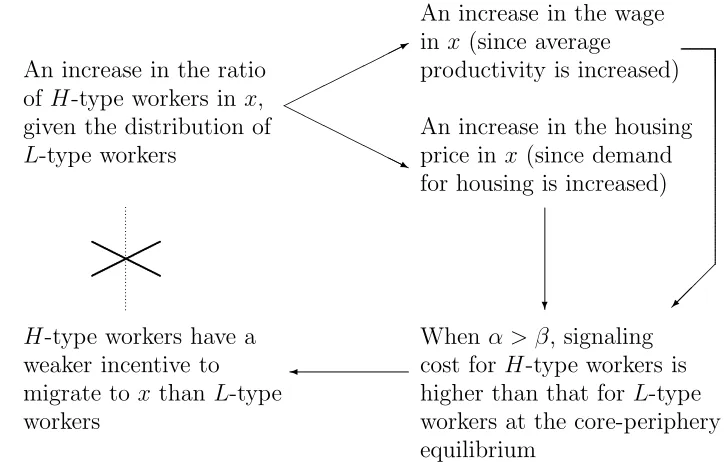
When α > β, signaling cost for H-type workers is higher than that forL-type workers at the core-periphery equilibrium
✛
[image:27.612.107.471.406.637.2]H-type workers have a weaker incentive to migrate to x than L-type workers
✲ ✛ ✻ ❄ ✛
✻ ❄
✲ ✻ ❄
✛
❄
✲ ✻
45◦ line
A
B E
˙ ρH = 0
˙ ρL= 0
0 1
1
ρH
ρL
Figure 3: When α = 2, β = 4, given nH = 1, nL = 2,¯s = 1, YL = 1,
and YH = 1.25, there exist two stable core-periphery equilibria, points A=
(0,0.61) and B = (1,0.39). In addition, since φH′
(ρH) < 0 at ρH = 1 2, the
completely symmetric equilibrium at point E = (1 2,
1
✛ ✲ ✻ ❄ ✛
✻ ❄
✲ ✻ ❄
✛
❄
✲ ✻
45◦
line
A
B
E
˙ ρH = 0
˙ ρL= 0
0 1
1
ρH
ρL
Figure 4: When α = 2, β = 4, given nH = 1, nL = 2,¯s = 1, YL = 1, and
YH = 2, there exist stable core-periphery equilibria at points A = (0,0.41)
✛ ✲ ✻ ❄
✛ ✻ ❄
✲ ✻ ❄
✲
✲ ✛
❄
✲ ✻
45◦
line
A
B
C
D
E ˙
ρH = 0 ˙ ρL= 0
0 1
1
ρH
ρL
Figure 5: When α = 2, β = 4, given nH = 1, nL = 2,¯s = 1, YL = 1,
and YH = 4, there exist three unstable integrated equilibria, points C =
(0.09,0.27), D= (0.91,0.73), and E = (1 2,
1
2), and there are two stable
✲ ✛ ✻ ❄ ✲
✻ ❄
✛ ✻ ❄
✛
❄
✲ ✻
45◦
line
˙ ρL= 0
˙ ρH = 0
E
0 1
1
ρH
ρL
Figure 6: When α = 4, β = 2, nH = 1, nL = 2,s¯ = 1, YL = 1 and
YH = 1.25, there exists a unique stable completely symmetric equilibrium;
✛ ✲ ✻ ❄
✲ ✻ ❄
✛ ✻ ❄
✛
❄
✲ ✻
45◦
line
E
˙ ρL = 0
˙ ρH = 0
0 1
1
ρH
ρL
Figure 7: When α = 4, β = 2, nH = 1, nL = 2,s¯ = 1, YL = 1 and
YH = 2, there exists a unique equilibrium which is completely symmetric
✛ ✲ ✻ ❄
✲ ✻ ❄
✛ ✻ ❄
✲
✲ ✛
❄
✲ ✻
45◦
line
C
D
E
˙ ρH = 0
˙ ρL= 0
0 1
1
ρH
ρL
Figure 8: When α = 4, β = 2, nH = 1, nL = 2,s¯ = 1, YL = 1 and
YH = 4, there exist three unstable integrated equilibria at C = (0.09,0.31),
D = (0.91,0.69), and E = (1 2,
1
2), respectively. In addition, there is no
✲
2 1.78
1.0 1
1 2
0 ρH
YH
Figure 9: The fork bifurcation when productivity and the elasticity of demand for land are positively correlated, given nH = 1, nL = 2, ¯s = 1,
YL = 1, α= 4, and β = 2.
2 1.56
1.0 1
1 2
0 YH
ρH
Figure 10: The fork bifurcation when productivity and the elasticity of demand for land are negatively correlated, given nH = 1, nL = 2, ¯s = 1,
![Table 1: Source: U.S. Census Bureau [1990], (CPH-2).](https://thumb-us.123doks.com/thumbv2/123dok_us/7919195.747173/26.612.110.487.274.406/table-source-u-s-census-bureau-cph.webp)