Supply Mix Optimization for Decentralized
Energy Systems
J. K. Gruber, J. L. Mínguez Fernández, M. Prodanovic
Electrical Systems Unit, IMDEA Energy Institute, Móstoles (Madrid), Spain
Email: [email protected], [email protected], [email protected] Received 2013
ABSTRACT
In recent years, the energy sector has undergone an important transformation as a result of technological progress and socio-economic development. The continuous integration of renewable energy sources forces a gradual transition from the traditional business model based on a reduced number of large power plants to a more decentralized energy produc-tion. The decentralization and the increased number of energy sources lead to a series of new challenges in the energy sector. This paper presents an approach to determine the optimal energy supply mix for small and medium sized build-ings or installations. The optimization algorithm considers the electricity and heat demand and determines the optimal combination of energy sources by minimizing an economic index. The optimization problem can be solved for multiple demand profiles and takes into account the possibility to integrate accumulator systems. The proposed approach pro-vides a high degree of flexibility and can be used to study the influence of the energy prices on the optimal energy sup-ply mix. The performance of the proposed optimization approach is illustrated by the results obtained from a simulation example.
Keywords: Energy Supply Mix; Optimal Configuration; Decentralized Generation
1. Introduction
The prosperity of modern societies is closely related to the availability of energy and the continuous supply is an important factor for the industrial development. In many countries a significant part of the energy demand is satis-fied with fossil fuels such as oil and gas or by means of nuclear power production. The constantly growing de-mand for fossil fuels and the shrinking reserves in com-bination with the necessary and more expensive modern extraction technologies lead to increased energy prices. Today, many economies depend highly on energy im-ports from a small group of countries with oil and gas reserves. The environmental impact of fossil fuels as well as the risks related to nuclear power generation gave rise to a serious discussion about the effects of traditional energy production. These drawbacks led in recent years to an increased research and development in alternative energy sources.
In recent years, the significant increase in the integra-tion of renewable energy sources compensated, at least to some extent, the problems related to the traditional en-ergy production. The continuous increase of alternative energy sources, especially wind turbines and photo-voltaic panels, emphasizes the change from a centralized energy production with few large power plants to a more
distributed generation. The power production near the place of consumption reduces the transmission losses, increases the energy efficiency and helps to ensure a high quality in the energy supply.
Nowadays, buildings contribute strongly to the total energy demand and account in some countries for up to 45% of the primary energy consumption [1, 2, 3]. A suit-able energy mix, especially the use of renewsuit-able energy sources, and an optimal supply system can improve the energy efficiency of buildings and reduce costs. The op-timal energy supply system for buildings in the tertiary sector is determined in [4] solving an economic minimi-zation problem by mixed integer linear programming (MILP). The algorithm in [5] considers both centralized and decentralized technologies and determines the opti-mal technology mix for a neighbourhood or a sopti-mall town taking into account constraints such as a maximum
emis-sion of CO2. The integrated approach presented in [6]
improves the energy efficiency combining the computa-tion of the optimal energy supply mix with a proactive energy management. The multi-objective optimization of an energy supply system for an industrial district [7] in-cludes the costs of the energy supply system and the
en-vironmental impact of a positive or negative CO2 balance
with respect to traditional systems.
special focus on the variability in energy production as a result of an increased wind power deployment. The au-thors underline the importance of storage systems which provide certain flexibility in the integration of intermit-tent energy sources. The prototype energy model pre-sented in [9] deals with the complex problem to consider social factors in the optimization of the energy supply mix. The approach translates energy policy goals, both quantitative and qualitative ones, into a set of mathe-matical expressions for the posterior optimization.
This paper presents a method to determine the optimal energy supply mix for small and medium sized buildings under consideration of seasonal profiles for electricity and heat demand. The optimization approach focuses on distributed energy generation in combination with elec-tric batteries and backup grid connection. The minimiza-tion of the objective funcminimiza-tion, an economic index based on the initial inversion and the generation costs, is car-ried out with sequential quadratic programming (SQP). The paper is organized as follows: Section 2 presents a detailed problem description and defines the objective function. The proposed approach for the minimization of the cost is given in Section 3. The implementation of the proposed optimization procedure and the obtained results for an office building are given in Section 4. Finally, in Section 5 the mayor conclusions are drawn.
2. Problem Description
This work presents an approach to determine the optimal energy supply mix for a small or medium sized building minimizing an economic index. The general objective
function J
x to be minimized is given by:
e
h
b
J x J x J x J x (1)
where xN denotes the vector with the installed
capacities and N is the total number of energy sources
considered in the cost function. The terms Je
xe
,
h and represent the costs related to the
electricity sources, the heat sources and the battery, re-spectively. The capacities are given by
J x
Jb
xN e
x for the
electricity sources, Nh
h x
, ,
T T
e h
for the heat sources and
b for the battery. The vector of capacities used in
(1) is defined as
x
T b x
x
x x
The cost related to the electricity sources is
defined as:
.
( )xe e
J
, ,
( ) ( ) ( )
e e e f e e v e
J x J x J x (2)
being , the annual fixed costs and , the
variable costs. The fixed costs Je f( )xe Je f, ( )xe are given by: Je v( )xe
( ) ( )
, ( )
1
( ) e
i i N
e e
e f e i
i e x I J y
x (3)
where ( )i e
x , ( )i e
I and ( )i
e
y are the installed capacity, the
necessary initial investment costs per installed capacity
and the technical lifetime of the i-th electricity source,
respectively. Note that the capacity ( )i
e
x corresponds to
the i-th element of the vector e. The variable
electric-ity costs are defined as:
x
( )i (i e , ( )
e v e J x
, e v
) 1
( ) e
N
e e e
i
J p se
x (4)
where ( )i
e
is the amount of energy of the i-th
electric-ity source consumed during a year and is the
cor-responding price per energy unit. The shortfall of electric energy is considered as an additional term based on the
amount of missing energy e
( )i e
p
s and the corresponding
penalization cost e per unit.
In the case of heating, the cost h( )xh is given by:
h v J J
,f( )h ,
( ) ( )
h h h h
J x J x
, h f J
x (5)
with the annual fixed costs and the variable
costs defined as:
(xh)
, ( ) h v xh J ( ) ( ) ( ) i i h h i h , ( )
h f h 1
h
N
i x I
( ) i i h J y x s
( ) h (6) , 1 ( ) h Nh v h h h
i
J p
x (7)
where ( )i h
x , ( )i h
I and yh( )i are the installed capacity, the
initial investment per installed capacity and the technical
life cycle of the i-th heat source, respectively. It is
im-portant to mention that ( )i
h
x is the i-th element of the
capacity vector xh. The variable h( )i denotes the amount
of energy of the i-th heat source consumed during a year
and is the price per energy unit. Besides, the
vari-able costs consider the case of a shortfall where h
( )i h
p
s
de-notes the amount of missing heat and h is the
penali-zation price of each energy unit. For the battery, the cost J xb( )b
, ( )b
is defined as:
,
( ) )
b b b f b v( b
J x J x J x
) b
(8)
with the fixed costs Jb f, (x and the variable costs
, ( b v b)
J x given by:
, ( ) b b
b b f b
x I y ( ) 1 e N b
J x (9)
( ) i i
e , ( )
b v b i
J x
p
(10)where xb denotes the installed battery capacity, Ib
represents the necessary initial investment per storage
capacity and b is the lifetime of the battery. The
vari-able costs depend on the amount of energy y
( )i b
from
the electricity sources used for battery charging and the
corresponding price ( )i per energy unit.
e
p
The amounts of consumed ( ( )i
e
, ( )i h
and b
( )i
) and
missing energy (se and sh) are determined during the
ca-pacities of the energy sources. The initial investments ( ( )i
e
I , ( )i h
I and Ib), the technical lifetimes ( ( )i
e
y , ( )i h
y and
b), the prices per energy unit ( and ) as well as
the costs for each missing energy unit (
y ( )i
e
p ( )i
h
p
( )i e
and ( )i
h
) are constant parameters and their values are known.
3. Optimization Procedure
The objective of the optimization procedure is to mini-mize the energy costs (1) for a given electricity and heat demand. The use of multiple profiles allows considering the variations in the demands throughout the year and provides a more realistic estimation of the energy costs. For a given set of capacities and given demand profiles, the chosen approach calculates the amount of energy consumed from each source and the amount of missing energy to satisfy the demand. The following sections explain in detail the use of the available energy sources to cover the demands.
3.1. Initial Considerations
Consider a sampling time of and the installed
capacities
1 h s
t
( )i e
x for i 1, ,Ne, xh( )i for i 1, ,Nh
and xb. Furthermore, consider the electricity and heat
profiles for a certain day given by the hourly demand
and with .
( e
d j)
j
( ) ( )j
, 2 ( ) i i e e h
The amount of energy which can be produced in each
sample by a source is given by the
expres-sions
d 0, , 23
s
j
0, 3 ( ) ( ) ( )
ei
g j f
( )
i i
h h
j x t
with i 1, ,Ne
and ( )( ) ( ) ( )
hi s
g j f j x t with i 1, ,Nh
where the parameters ( )i ( )
e
f j and ( )i
h ( )
f j are used to
consider external or internal influences on the energy production. For controllable energy sources, e.g. gas tur-bines, grid connection or biomass boiler, the possible
energy production is assumed to be ( )i ( )
e
f j 1 and
. In the case of the non-controllable energy sources, i.e. renewable sources such as wind turbines, photovoltaic panels or solar thermal collectors, the en-ergy production also depends on some environmental
conditions leading to and .
For controllable energy sources with simultaneous heat and energy production, e.g. combined heat and power
(CHP), the parameters e
( )i h ( )
f j 1
( ) 0 i e ( )( ) f j ( ) f j ( ) i i
1 0 f( )i (j) 1 h
and ( )
h
( ) ( ) i
f j i
with ( )i (i) 1 are used.
The operation modes of the considered battery does not admit simultaneous charging and discharging, i.e. in a given moment the battery represents either an energy source or an energy sink. Another limitation arises from
the power rate capabilities c and d for charging
and discharging, respectively. The amount of energy that can be drawn from or stored to the battery in each sample, without taking into account the current state of the
bat-tery, must not exceed v j
m
m m
c s ( )
c t and v jd( )md st
with j 0, , 23.
The considered capacities ( )i
e
x , ( )i h
x and xb allow
computing the fixed costs of the energy sources given by (3), (6) and (9). The variable costs (4), (7) and (10) have to be calculated after determining the amount of energy supplied by each source.
3.2. Assignment of Electricity Sources
The satisfaction of the energy demand using different sources is based on economic rules with the objective to minimize the costs. For a given set of installed capacities
x, priority is given to sources with a cheaper generation.
The optimization satisfies the electricity demand using an iterative procedure with the following assignment order: renewable sources, CHP and controllable sources. For simplicity of the notation and without loss of generality it is assumed that the electricity sources with the capacities
( )i e
x for i 1, ,Ne
(0)( ) ( )
e
r j d
are already sorted according to the sequence of assignment.
With the initially unsatisfied electricity demand given
by e j for j 0, , 23, in the i-th iteration
with i 1, ,Ne the amount of energy drawn from the
corresponding source is given by:
1)( ) ( )i( ),0 ,
0, , 23e
r j g j j
( )i( ) max (i
e e c j ( )( ) ( e e r j ( )( ) e e u j ( )
0, , 23
j
e
(11)
Then, the remaining unsatisfied demand becomes:
1)( ) ( )( ), 0, , 23
i i i
e
r j c j j
(12)
and the unused amount of energy which could be
pro-duced by the i-th energy source is:
( )( ) ( )( ), 0, , 23
i i i
e
g j c j j
(13)
Finally, finishing the iterative procedure, the total amount of energy generated by each source throughout an entire year can be calculated by:
23 ( ) 0
365 ( ), 1, ,
i i
e e
j
c j i N
(14)After using the energy sources, the remaining
electric demand for has to be
satisfied by the battery.
e
N
(Ne)( e
r j) j 0, , 23
3.3. Assignment of Battery
The battery is charged by means of the electricity sources using an iterative procedure and the previously described assignment order. Taking into account only the power rate limitations, the theoretical amount of energy that can be stored to the battery in a sample is
for
(0)( ) ( )
c c
w j v j
.
With the known initial state of charge and the
still unsatisfied demand for
(0) c
q j
( ) (0)( ) Ne ( )
b e
r j r j 0, , 23,
the amount of energy charged to the battery in the i-th
from the i-th source) is calculated as:
( )i( ) min ( )i ( ), ( )k , ( 1)
b e b c
c j u j x q wi
c (15)
if (0)( ) 0 and
b
r j ( )i ( ) 0 b
c j if with
and being a counter.
Evidently, charging will take place only in samples without demand, i.e.
(0)( ) 0 b
r j
0, , 23
j k j 24(i
(0)( ) 0 b
r j
1)
. After storing
in the battery, the remaining amount of energy that could be stored in a sample is given by:
( )i ( ) b
c j
( )i ( ) ( 1)i ( ) ( )i ( ), 0, , 23
c c b
w j w j c j j (16)
and the state of charge of the battery can be written as:
(k 1) ( )k ( )i ( ), 0, , 23
c c b
q q c j j (17)
The state of charge depends on the charging in
previous samples due to the recursive character of (17). As a direct consequence, (15)-(17) have to be evaluated
together for each sample in the i-th iteration.
(k 1) c
q
After charging the battery using the different energy
sources, the state of charge is given by (0) (24Ne)
d c
q q
and represents the initial state considered in the dis-charging procedure. The amount of energy drawn from the battery in each sample is defined as:
(0)
( ) min ( ), ( ), ( ) , 0, , 23
b b d d
z j r j q j v j j
e
(18)
The resulting unsatisfied demand after using the bat-tery can be written as:
(1)( ) (0)( ) ( ), 0, , 23
b b b
r j r j z j j (19)
and the amount of energy stored in the battery is:
( 1) ( ) ( ), 0, , 23
d d b
q j q j z j j (20)
Finally, after the charging and discharging procedures, the amount of energy taken from each source throughout the year and stored in the battery is given by:
23
( ) ( )
0
365 ( ), 1, ,
i i
b b
j
c j i N
(21)and the overall unsatisfied demand becomes:
23 (1) 0
365 ( )
e b
j r j
(22)3.4. Assignment of Heat Sources
The heat demand is covered step by step using an itera-tive procedure that gives priority to sources with a cheaper energy production. Based on this simple eco-nomic rule, the assignment order applied by the proce-dure is: renewable sources, CHP and controllable sources. For simplicity of the notation and without loss of gener-ality it is assumed that the considered heat sources with the capacities ( )i
h
x with are already sorted
in the given assignment order.
1, , h
i
Defining the initial heat demand as for
(0)( ) ( )
h h
r j d j
0, , 23
j , the amount of energy generated in the
i-th iteration by the corresponding source is given by:
( )i( ) max ( 1)i ( ) ( )i( ),0 , 0, , 23
h h h
c j r j g j j
h
j
(23)
with the generated energy , the remaining
unsat-isfied demand becomes:
( )i ( ) h
c j
( )i ( ) ( 1)i ( ) ( )i ( ), 0, , 23
h h h
r j r j c j j (24)
Finally, after finishing the iterative procedure the total amount of heat generated by each source during an entire year is given by:
23
( ) ( )
0
365 ( ), 1, ,
i i
h h
j
c j i N
(25)and the overall unsatisfied heat demand becomes:
23 ( ) 0
365 Nh ( )
h h
j r
(26)3.5. Cost minimization
The generated energy ( ( )i
e
, ( )i b
, ( )i h
) and the missing
energy (e,h) determined with the assignment
proce-dures are used to calculate the variable costs (4), (7) and (10). Furthermore, the fixed costs are given by (3), (6)
and (9) for a given set of capacities . Finally, the fixed
and variable costs allow computing the overall cost (1) related to the energy supply.
x
Now, the optimal capacities of the energy sources
are calculated solving the following minimization prob-lem under consideration of constraints:
* x
* arg min ( )
s.t.
J A
x
x x
x b (27)
with ANcN and bNc where
c denotes the
number of constraints. The optimization problem based on several iterative assignment procedures can then be solved with nonlinear programming (NLP).
N
4. Implementation & Results
The proposed approach for the minimization of the cost related to the energy supply of small and medium sized buildings has been implemented in Matlab. The optimal
capacities are computed solving the optimization
problem (27) with Matlab’s built-in function for sequen-tial quadratic programming (fmincon).
* x
4.1. Implementation
For the satisfaction of the electric demand, wind turbines, photovoltaic systems, gas turbines, CHP plants, grid connection and batteries have been considered. Heat pumps, oil boilers, CHP plants, solar thermal collectors
and biomass boilers have been taken into account for
heating. The technical lifetimes ( ( )i
e
y , ( )i h
y , ), the initial
investments per capacity unit ( b
y
( )i e
I , ( )i h
I ,Ib) and the
prices per energy unit ( , ) of the energy sources
are given in Table 1. In the case of an energy shortfall, a
penalization of
( )i e
p
10 ( )i h
p
00 €/kWh e h
is used for
elec-tricity and heat.
The parameters ( )i ( )
e
f j and ( )i ( )
h
f j
0.3
for photovoltaic and solar thermal systems located in Madrid (Spain) have been taken from the Photovoltaic Geographical
Informa-tion System (PVGIS) [10], see Figure 1. For wind
tur-bines an average performance of 30%, i.e. ,
has been assumed and for CHP systems the
electric-ity/heat ratio is given by and . For
all other electricity and heat sources,
( )i ( ) 0.3 e
f j
( )i 0.7
( )i ( ) 1 e
f j
( )i
and
have been used.
( )i ( ) 1 h
f j
Two demand profiles (see Figure 2), one for winter
and one for summer, have been used for the considered medium sized office building in Madrid. The optimiza-tion procedure of the energy supply mix considers half year of summer and half year of winter.
Table 1. Technical lifetimes, investments per capacity and energy prices of the considered energy sources.
Source Investment [€/kW] [€/kWh] Price Lifetime [a]
wind turbine 2400 0.04 20
photovoltaic system 4000 0.02 25
gas turbine 1200 0.08 10
CHP plant 1300 0.06 10
grid connection 15.97 0.12 1
battery 500 €/kWh − 5
geothermal heat pump 1500 0.07 20
oil boiler 600 0.08 10
solar thermal collector 1000 0.03 25
biomass boiler 350 0.08 20
Figure 1. Efficiency of the photovoltaic and solar thermal systems in summer (dash-dotted line) and in winter (solid line) and for the wind turbine in all seasons (dashed line).
4.2. Results
The implemented procedure was used to determine the optimal energy supply mix for the office building. The costs were optimized using current market prices (see
Table 1) for the different energy sources.
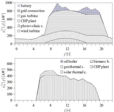
The obtained results of the energy consumption are
given for the summer profile in Figure 3 and for the
winter profile in Figure 4. It can be observed that that
the major part of the electricity and heat demands are covered by fossil energy sources and only a reduced proportion is satisfied by renewable energy. Furthermore, some of the available technologies are not included in the optimal energy mix (batteries, geothermal heat pumps, solar thermal collectors and oil boilers) due to economic reasons. The capacities of the energy sources and the amount of energy produced by each source are given in
Table 2. With the current prices, 82.7% of the energy demand is covered with fossil fuels, 5.2% is drawn from the grid and 12.1% is taken from renewable energy sources. In spite of the high capital costs of wind turbines
Figure 2. The considered electricity and heat demands for winter (solid line) and summer season (dashed line).
and photovoltaic systems, these sources satisfy 14.1% of the yearly electricity demand.
[image:6.595.58.289.192.419.2]With the continuously decreasing prices of renewable energy sources and the rising fossil fuel prices, decen-tralized generation will be more important in the future. Furthermore, it is expected that the improvements in storage technologies will reinforce the use of batteries and other accumulator systems.
[image:6.595.60.285.493.736.2]Figure 4. Satisfaction of the electricity (top) and heat de-mand (bottom) in winter.
Table 2. Capacities of the energy sources and amounts of energy generated during the year.
Source Capacity [kW] Annual gen. [MWh]
wind turbine 98.2 (6.0%) 258.0 (4.5%)
photovoltaic system 191.3 (11.6%) 392.2 (6.8%)
gas turbine 501.3 (30.4%) 2304.0 (39.9%)
CHP plant 593.2 (36.0%) 2469.1 (42.8%)
grid connection 191.2 (11.6%) 301.0 (5.2%)
battery 0 0
geothermal heat pump 0 0
oil boiler 0 0
solar thermal collector 0 0
biomass boiler 73.7 (4.5%) 46.4 (0.8%)
5. Conclusions
A procedure for the computation of the optimal supply mix for decentralized energy systems has been developed and implemented. The presented approach minimizes an objective function for a given energy demand using basic economic rules. The use of multiple profiles allows con-sidering seasonal variations in the electricity and heat demand. The described algorithm has been implemented in Matlab considering ten energy sources, including bat-teries and CHP systems. The optimization algorithm re-gards capital costs and variable costs resulting from the energy generation. Additional costs resulting from
de-commissioning, waste management, CO2 transport and
storage, fixed operating costs and others can be included easily in the minimization problem for a differentiated optimization and analysis of the supply mix.
The optimal energy supply mix for a medium sized of-fice building located in Madrid (Spain) was determined using the proposed optimization procedure. The obtained results showed a predominance of energy production from fossil fuels for current market prices and only a reduced use of renewable energy. The high flexibility of the procedure allows studying changes in the optimal energy supply in function of the investment costs and energy prices.
REFERENCES
[1] L. Pérez-Lombard, J. Ortiz and C. Pout, “A Review on Buildings Energy Consumption Information,” Energy and Buildings, Vol. 40, No. 3, 2008, pp. 394-398.
doi:10.1016/j.enbuild.2007.03.007
[2] J. Iwaro and A. Mwasha, “A Review of Building Energy Regulation and Policy for Energy Conservation in De-veloping Countries,” Energy Policy, Vol. 38, No. 12, 2010, pp. 7744-7755. doi:10.1016/j.enpol.2010.08.027
[3] A. H. C. dos Santos, M. T.W. Fagá and E. M. dos Santos, “The Risks of An Energy Efficiency Policy for Buildings Based Solely on the Consumption Evaluation of Final Energy,” International Journal of Electrical Power & Energy Systems, Vol. 44, No. 1, 2013, pp. 70-77.
doi:10.1016/j.ijepes.2012.07.017
[4] M. A. Lozano, J. C. Ramos, M. Carvalho and L. M. Serra, “Structure Optimization of Energy Supply Systems in Tertiary Sector Buildings,” Energy and Buildings, Vol. 41, No. 10, 2009, pp. 1063-1075.
doi:10.1016/j.enbuild.2009.05.008
[5] C. Weber and N. Shah, “Optimisation Based Design of A District Energy System for An Eco-town in the United Kingdom,” Energy, Vol. 36, No. 2, 2011, pp. 1292-1308.
doi:10.1016/j.energy.2010.11.014
[7] D. Buoro, M. Casisi, A. De Nardi, P. Pinamonti and M. Reini, “Multicriteria Optimization of A Distributed En-ergy Supply System for An Industrial Area,” Energy, 2013. doi:10.1016/j.energy.2012.12.003
[8] C. De Jonghe, E. Delarue, R. Belmans and W. D’haeseleer, “Determining Optimal Electricity Technol-ogy Mix with High Level of Wind Power Penetration,”
Applied Energy, Vol. 88, No. 6, 2011, pp. 2231-2238.
doi:10.1016/j.apenergy.2010.12.046
[9] A. Chee Tahir and R. Bañares-Alcántara, “A Knowledge Representation Model for the Optimisation of Electricity Generation Mixes,” Applied Energy, Vol. 97, 2012, pp. 77-83. doi:10.1016/j.apenergy.2011.12.077