The Realization and Working Conditions of Memristor Based on Multisim

(1)

The Realization and Working Conditions of Memristor

Based on Multisim

*

Dehua Song1, Xiang Ren1, Mengfei Lv1, Mengmeng Li1, Haiyang Zhou1, Yunxiao Zu2

1

School of Information and Telecommunication Engineering, Beijing University of Posts and Telecommunications, Beijing, China; 2

School of Electronic Engineering, Beijing University of Posts and Telecommunications, Beijing, China. Email: [email protected]

Received July 2013

ABSTRACT

An equivalent circuit is realized using Multisim software by transforming a kind of circuit element according to Map- ping principle and circuit theory. The effects of every parameter on the equivalent circuit are analyzed and the working conditions of the equivalent circuit are concluded by simulation.

Keywords: Memristor; Multisim; Equivalent Circuit; Realization; Working Conditions

1. Introduction

Four researchers from HP laboratory successfully manu- factured memristor based on the metal and metal oxide in Nano-scale in 2008 and found the mathematical model of memristor [1]. The memristor was being focused since then [2-11]. However, analysing the circuit containing memristor is very difficult because the voltage-current relation (VCR) of memristor is a multivalued function. Though researchers usually use a linearization approach to analyse the circuit, it is also difficult and inaccurate. A mutator converting other circuit components into memristors is built in this paper according to the mapping principle and circuit theory based on Multisim in order to analyse circuit containing memristor easily and accu- rately.

Memristor is an element which provides a functional relation between flux linkage ψ and charge q, and the basic model is as follows.

dψ =M qd (1) where M is the memristance of the memristor.

2. Circuit of Mutator

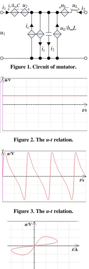
Mutator converts VCR of an element into Ψ-q relation to simulate memristor. The circuit of mutator is shown in

Figure 1.

The Realization of Memristor Based on Multisim

Assigning hm = 0.4, km = 1000, L = 1 mH, C = 1 mF, R =

1 Ω, I = 1 A. The u-t relation of memristor is shown in

Figure 2 by simulation in Multisim. The longitudinal axis scale is 500 V/Div. It can be seen that the curve is a straight line paralleled with axis t, so the memristor is equivalent to a linear resistor.

Memristor with fixed M is converted by linear resistor, so no research value. Only M is variable can memristor has memory function, so a nonlinear component as the converted component is necessary. The diode can be converted a memristor with variable M. Because the VCR cannot be shown directly in Multisim, a 1 Ω resistor is in series in the circuit. In this way, the current of the circuit can be detected because the voltage and the current of the 1 Ω resistor are numerically equal. The channel A of the oscilloscope is used to detect the voltage of memristor while the channel B is used to detect the voltage of 1 Ω resistor, then the VCR can be obtained using the A/B mode.

The VCR of the equivalent memristor can be obtained when the sine alternating current i = sin(2πƒt)A, ƒ = 1 kHz is added on the circuit and let hm = 0.4, km = 1000, L = 1 mH, C = 1 mF. The u-t relation is shown in Figure 3. The horizontal axis scale is 500 us/Div and the longitudinal axis scale is 500 mV/Div. The VCR of memristor is shown in Figure 4. Both the horizontal axis scale and the longitudinal axis scale are 500 mV/Div. It can be seen that the VCR of the equivalent memristor is an inclined “8” and very close to the VCR in literature [2]. So the circuit can be as the equivalent memristor with little error.

The circuit of converting the diode into memristor in

(2)

u1

ic i2

uL/hmL

[image:2.595.99.542.67.561.2]

Figure 1. Circuit of mutator.

[image:2.595.313.539.80.506.2]

Figure 2. The u-t relation.

Figure 3. The u-t relation.

Figure 4. The VCR of the equivalent memristor.

Multisim is shown in Figure 5.

3. The Working Conditions of the

Equivalent Circuit

3.1. The Influences of hm and km

Put

m

u k

i h q

ψ =   =

 (2)

into the VCR of the diode _se t

u U

i=I , Equation (3) can be gotten.

se

m t k

U m

h q I

ψ

[image:2.595.100.248.83.529.2]

= (3)

Figure 5. The simulation circuit in Multisim.

Simplifying Equation (3)

t s

ln

m m

k h q

U I

ψ ₌ ₍₄₎

Making differential on t in both sides of Equation (4).

s

t s

d d

m m

m

k I h q

U t h q I t

ψ ₌

(5)

Put d , d

d d

q

u i

t t

ψ

= = into Equation(4).

t 1 m

k

u i

U =q

(6)

Put

0 d

t

q=

∫

i t into Equation (6).

t

d t m

U i

u

k _{i t}

−∞

=

∫

(7)

Analyzing Equation(7) and can found that with the same current, the bigger hm, the smaller the voltage and the resistance of the equivalent circuit. Assigning Is = 0.1 uA, Ut = 26 mV, i = sin(2πƒt)A, ƒ = 1 kHz, hm = 1, then the u-t relation for different km in MATLAB simulation is shown in Figure 6.

It can be seen from Figure 6 that the voltage peak varies with different km. The bigger km, the smaller the voltage peak will be. Although the changing rate of the voltage is variable, the u-t relations for different km have not intersected except the origin. Because the value of the current source is the same at same moment, the bigger the voltage, the bigger the resistance of the equivalent circuit, and at different moment the resistance is bigger for smaller km.

The simulation waveform is the same with that of theoretical analysis. For the same current source, the smaller

[image:2.595.308.537.86.247.2]

(3)

Figure 6. The u-t relation for different km.

approaches to a straight line and closes to i axis when km increasing, while the shape of the u-t curve does not change but the voltage peak decreasing. Assigning km = 5000, hm = 0.4, and the VCR of the equivalent circuit is shown in Figure 7, in which both the horizontal axis scale and the longitudinal axis scale are 500 mV/Div. Increasing km until the oscilloscope can not display, however the shape of VCR still remains the same. Decreasing

km, the VCR of the equivalent circuit gradually approaches to a straight line and closes to u axis. When km changes very little, the shape of u-t curve does not change but the voltage peak increasing. When km is smaller than 10-7, the u-t curve of the equivalent circuit approaches to the sinusoid and shows the properties of linear resistor rather than memristor with changing me- mrisistance. Assigning km = 10−7，hm = 0.4, and the u-t relation of the equivalent circuit is shown in Figure 8, and in which the horizontal axis scale is 500 us/Div and the longitudinal axis scale is 500 MV/Div. It can be seen that the curve is very close to sinusoid. Because some elements of the equivalent circuit are active elements, the circuit takes some time to get stable, the stability of the circuit will not be changed when changing km, that is the VCR curves will never overlap. In a word, when hm = 0.4, the error of the circuit is small if km is between 10 and 104.

The impact of hm on the equivalent circuit is different from that of km. For the same current source, the time the voltage in the u-t curve reaching zero is the same for different hm, and that is right for the voltage reaching the peak. hm has no impact on the time the voltage reaching the peak. The simulation waveform in Multisim is different from that of the theoretic analysis. For the same current source, the bigger hm, the bigger the voltage peak will be. That is mainly because the VCR of the diode is only approximately exponential. Assuming

( )

u= f i (8)

Put Equation (2) into Equation (8), do differential both sides of Equation (8) and simplify it.

0 '( t d ) m

m m

h

u f h i t i

k

=

_∫

(9)

Figure 7. The VCR when km = 5000.

Figure 8. The u-t relation when km = 10−7.

It can be seen that if VCR is not standard exponential relationship, the equivalent circuit will be affected by hm.

Assigning L = 1 mH, C = 1 mF, i = sin(2πƒt)A and ƒ = 1 kHz. When hm is not largely changed, only the voltage peak in the u-t curve increasing, while the shape of the curve does not changing. When hm is bigger than 104, the shape of the u-t curve will obviously change, the voltage peak is not being constant, the voltage near the peak varies very quickly and the maximum positive value and the maximum negative value is not equal. Assigning km = 1000, hm = 104, the u-t curve of the equivalent circuit is shown in Figure 9. The scales of the horizontal axis and the longitudinal axis are 500 us/Div and 5 V/Div respectively. It can be seen that the u-t relation is no longer periodic.

In the same way, increasing hm, the u-i curve of the equivalent circuit changes a lot, from a convex and oblique “8” changes to a concave and oblique “8”, which is quite different from the u-i curve in literature [1]. Figure 10 is the u-i curve when km = 1000, hm = 104. Both the scales of the horizontal axis and the longitudinal axis are 1 V/Div. It can be seen that the curve obviously twists and different from the curve in Figure 4. Figure 11 is the amplified curve partially by changing the scale of the horizontal axis to 10 V/Div and the longitudinal axis to 50 mV/Div. It can be seen that the u-i curve is composed of many intersected curves. So when hm = 104, the equivalent circuit is no longer stable and changes in every period of the current source, which is also why the voltage peak in Figure 10 is a fixed value.

(4)

Figure 9. The u-t curve when hm = 104.

Figure 10. The u-i curve when hm = 104.

Figure 11. The amplified u-i curve when hm = 104.

shown in Figure 12. Both the horizontal axis scale and the longitudinal axis scale are 500 mV/Div. The u-t curve is shown in Figure 13, the scales of the horizontal axis and the longitudinal axis are 1 ms/Div and 200 mV/Div respectively. It can be seen that the voltage peak changes less than that of Figure 3. When hm is not largely changed, only the voltage peak of the u-t curve decreases, the shape of the curve doesn’t change much and the curve gets smoother. When hm is smaller than 0.01, the

u-t curve significantly changes and closes to the normal sinusoid. Assigning km = 1000, hm = 0.1, the u-t curve is shown in Figure 14, the horizontal axis scale is 500 us/Div and the longitudinal axis scale is 50 mV/Div. It can be seen that the curve is very close to normal sinu-soid, while the u-i curve of the equivalent circuit is close to a straight line, the circuit shows the characteristic of linear resistor rather than memristor with changing me-mrisistance. The stability of the circuit will not be af-fected when hm decreases. So when km = 1000, hm = 0.01 ~ 104, the error of the equivalent circuit is small.

3.2. The Influences of C and L

It can be seen from Equation (7) that the capacitor and inductor have no influences on the equivalent circuit. The

Figure 12. The u-i curve when hm = 0.1.

Figure 13. The u-t curve when hm = 0.1.

Figure 14. The u-t curve when hm = 0.01.

simulation result is the same with that of the theoretical analysis. Although the capacitance and inductance in the equivalent circuit are adjustable, the curves of VCR and

u-t don’t change with the capacitance and inductance. When the inductance is in a certain range, assigning i =

sin(2πƒt)A, ƒ = 1 kHz, hm = 0.4, km = 1000, changing the capacitance or inductance respectively, the curves of VCR and u-t are totally the same with that of Figure 3

and Figure 4, which shows that the capacitor and inductor have no influences on the equivalent circuit. However, when the inductance is bigger than 1 mH, there will be errors in simulation. Though simulation can be continued by cutting down the peak value of current source, the u-i

curve is close to a straight line and the u-t curve is close to sinusoid because of the too small current. So the circuit shows the characteristic of linear resistor and cannot represent memristor. Such simulation circumstances won’t happen when changing the capacitance.

3.3. The Influences of the Source’s Peak and Frequency

It can be seen from Equation (7) that the current source’s peak has impact on the VCR and u-t relation of the equivalent circuit. Put i = Isin(2πƒt) into Equation (7) and simplify it.

m

2 sin(2 )

cos(2 ) 1 t

U f ft

u

k f

π π

π =

− (10)

(5)

peak, the flatter the u-i curve, and closer to the horizontal axis.

Assigning i = Isin(2πƒt)A, ƒ = 1 kHz, hm = 0.4, km = 1000, L = 1 mH, C = 1 mF. When I = 10 A the u-i curve is shown in Figure 15, the scales of the horizontal axis and the longitudinal axis are 5 V/Div. It can be seen that the curve is very close to the horizontal axis. When the current peak I is bigger than 50 A, the stability of the equivalent circuit weakens and the u-t curve loses peri- odicity. When I = 50 A the u-i curve is shown in Figure 16, the scales of the horizontal axis and the longitudinal axis are 2 V/Div. It can be seen that the equivalent circuit is very unstable, many curves lap over, and the analysis result of the circuit is not accurate. When decreasing the current, the u-i curve is close to a straight line. However, the slope k of the curve keeps constant when changing the current value. This is mainly because that the current value is so small that the resistance of the equivalent circuit varies less and can be approximately regarded as a linear resistor in a short period. For example, when I = 0.01 A the u-i curve is shown in Figure 17. The scales of the horizontal axis and the longitudinal axis are 10 mV/Div. It can be seen that the u-i curve is very close to a straight line. So the circuit shows the characteristic of linear resistor and the characteristic of memristor is not obvious. However, the stability of circuit will not be affected when decreasing the current. In a word, the circuit is not stable if the current is very big, and the circuit will show the characteristic of linear resistor if the current is over-small. So the equivalent circuit in Figure 1 can simulate the memristor only when the effective value of the current is 0.01 ~ 50 A.

Figure 15. The VCR when I = 10 A.

Figure 16. The u-i curve when I = 50 A.

Figure 17. The u-i curve when I = 0.01 A.

It can be seen from Equation (10) that the frequency of the current source has impact on the VCR and u-t curve of the equivalent circuit. Assigning i = sin(2πƒt)A, hm = 0.4, km= 1000, L = 1 mH, C = 1 mF. Increasing the frequency of current source in a certain range, the u-t curve doesn’t change obviously, and the node of the oblique “8” of the u-i curve offsets upward but not so obviously.

Assigning f = 100 kHz, the u-i curve of the equivalent circuit is shown in Figure 18. The scales of the horizon-tal axis and the longitudinal axis are 500 mV/Div. It can be seen that the u-i curve is no longer an oblique “8” but an oval, the circuit is unstable, and the curve is composed of many curves. The u-t curve of the equivalent circuit is shown in Figure 19. The scales of the horizontal axis and the longitudinal axis are 10 us/Div and 500 mV/Div respectively. It can be seen that the curve is close to sinusoid, the voltage peak is bigger in the first cycle of the current source, and then the voltage peak gets to stable, so the stability of circuit gets less. When decreasing the frequency of the current source, the u-i curve gets flatter and closes to the horizontal axis, and the characteristic of the equivalent circuit approaches to the linear resistor. The u-t curve has not obviously change. Assigning f = 100 Hz, the u-i curve of the equivalent circuit is shown in

Figure 20. The scales of the horizontal axis and the longitudinal axis are 500 mV/Div. It can be seen that the curve is very similar to Figure 16. In a word, if the frequency is over high, the u-i curve of the equivalent circuit is obviously distorted and the circuit is unstable, and

Figure 18. The u-i curve when ƒ = 100 kHz.

Figure 19. The u-t curve when ƒ = 100 kHz.

(6)

4. Conclusion

A mutator is built based on Multisim as an equivalent circuit of memristor in this paper. The parameters which impact on the equivalent circuit are analyzed, and the working conditions of the equivalent circuit of memristor are given. The errors of the equivalent circuit are smaller when km is 10 ~ 104 and hm is 0.01 ~ 104, the inductor and capacitor have no effects on the equivalent circuit when L < 1 mH, the frequency should be ƒ < 10 kHz, and the current should be I < 50 A. Which means the circuit can not be used in high frequency circuit.

5. Acknowledgements

The work is supported by the Research Innovation Fund for College Students of Beijing University of Posts and Telecommunications.

REFERENCES

[1] D. B. Strukov, G. S. Snider, D. R. Stewart and R. S.Williams, “The Missing Memristor Found,” Nature, Vol. 453, 2008, pp. 80-83.

[2] X. Zhang, Y. Z. Zhou, Q. Bi, X. H. Yang and Y. X. Zu, “The Mathematical Model and Properties of Memristor with Border Constraint,” Acta Physica Sinica, Vol. 59, No. 9, 2010, pp. 6669-6676.

[3] Q. H. Wang and W. P. Song, “Realization of Memristor by Two-Port Mutator,” Journal of Electrical & Electronic Education, Vol. 33, No. 3, 2011, pp. 56-57.

[5] Y. Zhang, X. L. Zhang and J. B. Yu, “Approximated SPICE Model for Emristor,” International Conference on Communications, Circuits and Systems, 2009, pp. 928- 931.

[6] D. P. Wang, Z. H. Hu, X. Yu and J. B. Yu, “A PWL Model of Memristor and Its Application Example,” In-ternational Conference on Communications, Circuits and Systems, 2009, pp. 932-934,

[7] Klaus Witrisal, “A Memristor-Based Multicarrier UWB Receiver,” Proceedings of IEEE International Conference on Ultra-Wideband, IEEE Press, Sep. 2009, pp. 678-683,

[8] D. Varghese and G. Gandhi, “Memristor Based High Linear Range Differential Pair,” International Conference on Communications, Circuits and Systems, Jul. 2009, pp. 935-938.

[9] A. Delgado, “Input-Output Linearization of Memristive Systems,” Proceedings of IEEE Nanotechnology Mate-rials and Devices Conference, IEEE Press, July. 2009, pp. 154-157.

[10] M. Di Ventura, Y. V. Pershin and L. O. Chua, “Circuit Elements with Memory: Memristors, Memcapacitors, and Meminductors,” Proceedings of IEEE, Vol. 97, Oct. 2009, pp. 1717-1724.

[11] L. O. Chua, “Memristor—The Missing Circuit Element,” IEEE Transactions on Circuit Theory, Vol. 18, Sep. 1971, pp. 507-519.