Munich Personal RePEc Archive
Endogenous technological progress and
the cross section of stock returns
Lin, Xiaoji
London School of Economics and Political Science
15 January 2009
Endogenous Technological Progress and the
Cross Section of Stock Returns
Xiaoji Lin
yLondon School of Economics and Political Science
January 2009
Abstract
I study the cross sectional variation of stock returns and technological progress using a dynamic equilibrium model with production. In the model, technological progress is en-dogenously driven by R&D investment and is composed of two parts. One part is product innovation devoted to creating new products; the other part is dedicated to increasing the productivity of physical investment and is embodied in new tangible capital (e.g., structures and equipment). The model breaks the symmetry assumed in standard models between in-tangible capital and in-tangible capital, in which the accumulation processes of in-tangible capital stock and intangible capital stock do not a¤ect each other. The model explains qualitatively and in many cases quantitatively well-documented empirical regularities: (i) the positive relation between R&D investment and the average stock returns; (ii) the negative relation between physical investment and the average stock returns; and (iii) the positive relation between book-to-market ratio and the average stock returns.
JEL Classi…cation: E23, E44, G12
Keywords: Technological Progress, R&D Investment, Physical Investment, Stock Return
This paper is based on chapter one of my doctoral dissertation at the University of Minnesota. I am grateful to my committee members Frederico Belo, John Boyd, Murray Frank, Tim Kehoe, especially Robert Goldstein (chair) and Lu Zhang for their valuable advice and continuous encouragement. I thank Antonio Bernardo, Laurent Fresard, John Kareken, Sam Kortum, Ellen McGrattan, Pedram Nezafat, Monika Piazzesi, Lukas Schmid (WFA discussant), Chun Xia, and Suning Zhang for their comments. I thank the seminar participants at the Arizaona State University, Indiana University, London School of Economics and Political Science, NYU Stern, University of Michigan, University of Minnesota, University of Toronto, University of Washington at Seattle, and the 2007 FMA Doctoral Students Consortium and the WFA 2008. I acknowledge the support of the Carlson School Dissertation Fellowship. I thank the Western Finance Association for awarding this paper the Tre¤tzs Award in 2008 Waikoloa meetings. All errors are my own.
yDepartment of Finance, London School of Economics, Houghton Street, London WC2A 2AE, U.K. Tel:
1
Introduction
This paper investigates intangible capital, tangible capital and the cross section of stock returns
using a dynamic equilibrium model. The primary type of intangible capital the paper focuses on
is the accumulation of …rms’ research and development (R&D) e¤orts.1 The central insight of
the paper is that physical capital embodied-technological progress is essential to simultaneously
explaining the well-documented puzzling facts regarding R&D investment and physical investment:
i) high R&D-intensive …rms earnhigher average stock returns than low R&D-intensive …rms [e.g.,
Chan, Lakonishok and Sougiannis 2001; Li 2006]2; and ii) high physical investment-intensive …rms
earn lower average stock returns than low physical investment-intensive …rms [e.g., Titman, Wei
and Xie 2004; Xing 2008]3.4 Moreover this paper directly links technological innovation to the
di¤erences between the value and the growth …rms. Hence it provides a fresh explanation for the
value premium, which is di¤erent from the existing literature.
Indeed, the positive covariation between R&D investment and expected stock returns is
puz-zling for the neoclassical Q-theory of investment. As shown by Cochrane (1991), under constant
returns to scale stock returns equal investment returns. Since investment negatively forecasts
expected investment returns, it must also be negatively correlated with expected stock returns.
However, this prediction is inconsistent with R&D’s positive forecasting of expected stock returns.
Standard models cannot simultaneously explain the di¤erent covariations between R&D
in-vestment, physical investment and expected stock returns. For example, Hansen, Heaton and
Li (2004) and McGrattan and Prescott (2005) treat tangible capital and intangible capital
sym-metrically. More speci…cally, in their respective models, the accumulation processes of tangible
capital stock and intangible capital stock do not a¤ect each other. However, these models predict
that R&D investment and physical investment forecast future stock returns in the same direction,
1Tangible capital consists primarily of equipment, machines, and plants, which is usually labelled as physical
capital. Throughout the paper I use tangible and physical interchangeably, and intangible and R&D interchangeably as well.
2At aggregate level, Hsu (2006) …nds that aggregate cumulative R&D growth rate positively forecasts future
stock market returns.
3Cochrane (1991) and Lamont (2000) …nd that aggregate physical investment also negatively forecasts future
stock market returns.
4These …ndings regarding R&D investment and physical investment still hold after controlling for size and
which is counterfactual.
Three basic assumptions underpin the model. The …rst assumption is that technological
progress is endogenously driven by R&D investment. This assumption is familiar from Romer
(1990) who argues that technological progress largely arises from …rms’ R&D investment
deci-sions. In the model, I assume technological progress is a result of …rms’ explicit R&D decisions
and is represented by intangible capital. Here, intangible capital primarily refers to successful
innovations in advances in manufacturing technologies and processes, new designs and formulas
that generates new products, etc.
The second assumption is that part of the …rms’ technological progress is devoted to new
products. This assumption comes from R&D literature. Cohen and Klepper (1996) and Lin and
Saggi (2001) document that a large proportion of …rms’ R&D expenditures are used in
innova-tions to generate new products. For example, in pharmaceuticals, software companies, etc., more
than half of the total R&D expenditures are dedicated to new product innovations. Typically,
product innovation increases …rms’ cash ‡ows through the introduction of new product features
that increases the price buyers are willing to pay for …rms’ products, or allows …rms to reach new
buyers5. In the model, product innovations combined with physical capital produce products.
The third assumption, which is the key assumption in the paper, is that the other part of
technological progress is innovation devoted to increasing the productivity of physical investment
in producing new physical capital. Hence, in the model, the advances of new physical capital
embody current technological progress. This assumption is crucial to simultaneously generate a
positive covariation between R&D investment and future stock returns, and a negative covariation
between physical investment and future stock returns. The assumption of embodiment captures
the fact that successful innovations increase the productivity of equipment and machines and
reduce the costs of production process (Levin and Reiss 1988, Cohen and Klepper 1996). For
instance, in petroleum re…ning, biochemical industry, etc., more than two thirds of the total R&D
expenditure is dedicated to innovations in reducing production costs. Likewise, a number of other
industries, including petrochemicals, food and beverage manufacturing, semiconductor plants,
invest R&D in manufacturing technology for designing, analyzing and controlling manufacturing
through timely measurements (during processing) of critical quality and performance attributes
of raw and in-process materials and processes, with the goal of ensuring …nal product quality.
The main economic implications of the model are as follows. First, …rms’ expected returns
on physical investment are increasing in R&D investment butdecreasing in physical investment.
Intuitively, expected physical investment return is the ratio of the expected marginal bene…t of
physical investment to the marginal cost of physical investment. All else being equal, on one hand,
R&D investment increases the expected marginal bene…t of physical investment; on the other
hand, R&D investment (physical investment) decreases (increases) the marginal cost of physical
investment. These two e¤ects reinforce each other and imply that R&D investment (physical
investment) increases (decreases) expected returns on physical investment.
The second economic implication is that high R&D-intensive …rms earn higher expected stock
returns than low R&D-intensive …rms, while high physical investment-intensive …rms earn lower
expected stock returns than low physical investment-intensive …rms. Intuitively, in the model, the
stock price is the sum of the market value of physical capital and R&D capital, and the stock
return is the weighted average of physical investment return and R&D investment return. Since
physical capital embodies current technological progress (R&D capital) and its share in output
production dominates that of R&D capital, the market value of physical capital is higher than the
market value of R&D capital. This relation implies that the weight on physical investment return
is greater than the weight on R&D investment return.6Therefore, …rms’ stock returns covary with
R&D investment and physical investment in the same way as physical investment returns do. The
implication is that stock returns are increasing in R&D investment but decreasing in physical
investment.
The third economic implication is that value …rms earn higher expected stock returns than
do growth …rms7. Intuitively, with high book-to-market ratio, value …rms have low physical
investment, which implies that they must earn high expected physical investment returns. Growth
6In the model, the weight on physical (R&D) investment return is the ratio of the market value of physical
(R&D) capital to the stock price.
7An incomplete list of studies exploring why book-to-market ratio positively forecasts average stock returns
…rms have low expected physical investment returns because they have high physical investment
with low book-to-market ratio. Hence, value …rms earn high expected stock returns while growth
…rms earn low expected stock returns because the weight on physical investment return is larger
than the weight on R&D investment return. More speci…cally, in the model, the productivity of
the existing physical capital of value …rms is lower than that of growth …rms, because value …rms
invest less in R&D. In recessions, value …rms are burdened with excessive physical capital and
do not have as much technological progress in upgrading the e¢ciency of the existing physical
capital as do growth …rms, so they are more risky given that the market price of risk is high
in bad times. The value premium in my model hinges on the interactions between technological
progress and physical investment, which di¤ers from Zhang (2005) who work through physical
capital adjustment costs in generating the value premium. Given that most of the studies on
book-to-market ratio and stock returns focus on physical investment only, this paper sheds light
on the relation between technological progress and the value premium.
Cochrane (1991, 1996) are the …rst to study asset prices from …rms’ perspective using the
Q-theory of investment. Di¤erent from Cochrane who focuses on aggregate physical investment
and expected stock returns, this paper explores the relations between …rms’ technological progress,
physical investment and the cross-section of returns.
Li (2006) has a paper close to mine. In it Li constructs a dynamic real options model in which
R&D investment and stock returns change in predictable ways when R&D …rms are …nancially
constrained. The key distinction between Li and my model is that the real option model of Li
features exogenous cash ‡ows, systematic risk and …nancing constraints; while my model employs
a neoclassical framework in which technological progress is endogenously determined. Hence, in
my model the key economic fundamental variables, i.e., R&D investment, physical investment and
stock returns, are determined endogenously in competitive equilibrium. My model can therefore
shed light on the fundamental determinants of technological progress, and the covariations between
R&D investment, physical investment and future stock returns without resorting to …nancing
frictions.
…rm level, but with a di¤erent focus than this paper. Lustig, Syverson and Van Nieuwerburgh
explores the implications of IT adoption on corporate payout, organizational capital and changes
in labor market reallocation, while this paper examines the implications of …rms’ technological
change on asset prices and returns.
2
A Two-Period Example
I use a simple two-period example to provide intuition for the link between expected returns and
…rm characteristics.
2.1
The Setup
2.1.1 Technology
Firms use physical capital, intangible capital and a vector of costlessly adjustable inputs to produce
output. Firms choose the levels of these inputs each period to maximize their operating pro…ts,
de…ned as revenues minus the expenditures on these inputs. Taking operating pro…ts as given,
…rms then choose optimal physical investment and R&D investment to maximize their market
value.
There are only two periods, t and t + 1. Firm j starts with physical capital stock km j;t and
intangible capital stock ku
j;t, invests in periodt, and produces in botht andt+ 1. Physical capital,
including structures, equipment and machines, can be measured. So I denote it withm. Intangible
capital, including innovations in designs and formulas, new technologies in manufacturing, etc., can
be unmeasured. So I denote it withu. The …rm exits at the end of periodt+ 1with a liquidation
value of (1 m)kmj;t+1+ (1 u)kuj;t+1, in which m and u are rates of depreciation for physical
capital and intangible capital, respectively. Operating pro…ts, (km
j;t; kuj;t; j;t), depend upon
physical capital, km
j;t, intangible capital stock, kuj;t;where is the proportion of intangible capital
devoted to producing new products with0 <1, and a vector of exogenous aggregate and
…rm-speci…c productivity shocks, denoted as j;t. Operating pro…ts exhibit constant returns to scale
in km
subscripts mand udenote partial derivatives w.r.t. km
j;t andkj;tu :The expression m(kmj;t; kj;tu ; j;t)
is therefore the marginal product of physical capital, and u(kj;tm; kuj;t; j;t)is the marginal product
of intangible capital.
In the rest of the paper, I drop the …rm indexj when no confusion results.
2.1.2 Intangible Capital and Tangible Capital Production
As is standard in the literature, intangible capital production follows the standard capital
accu-mulation process given by
ktu+1 = (1 u)kut +iut; (1)
whereiut is R&D investment. Standard models also commonly assume that physical capital follows
a symmetric process, km
t+1 = (1 m)kmt +imt ; whereimt is physical investment.8
However, specifying physical capital and intangible capital symmetrically produces a model
that predicts that both R&D investment and physical investment forecast expected stock returns
in the same direction, which is counterfactual. I therefore abandon the symmetry of standard
models and specify the following accumulation process for physical capital
ktm+1 = (1 m)ktm+ imt ;(1 )kut+1 ; (2)
where
imt ;(1 )ktu+1 A a(imt ) + (1 a) (1 )kut+1
1
:
(3)
is a constant-elasticity-of-substitution (CES) technology for physical capital production.
Here,fa; ; Agare constants with the constraints0< a 1; 1; 6= 0;andA >0. Note that (1 )ku
t+1is the proportion of intangible capital dedicated to producing new physical capital. The
CES function im
t ;(1 )ktu+1 in equation (2) generalizes the standard accumulation process
as a special case when A=a= = 1:9 It satis…es
1 imt ;(1 )kut+1 > 0; 2 imt ;(1 )ktu+1 >0;
11 imt ;(1 )kut+1 < 0; 12 imt ;(1 )kut+1 >0; and 22 itm;(1 )ktu+1 <0;
where numerical subscripts denote partial derivatives. That is, the total product of physical capital
increases in the level of physical investment and intangible capital; moreover, the marginal product
of physical investment decreases in physical investment but increases in intangible capital, and the
marginal product of R&D capital decreases in R&D capital but increases in physical investment10.
The elasticity of substitution between ku
t+1 and imt is 11 :
The most important aspect of equation (2) is the inclusion of the intangible capital(1 )ku t+1
that represents the current state of technological progress for producing new physical capital.
A high realization of (1 )ku
t+1 increases the productivity of physical investment and directly
upgrades the e¢ciency of physical capital from the current vintage to the next. The increases in
(1 )ku
t+1 formalizes the notion of embodied technological progress.
The motivations for equation (2) come from the macro literature on embodied technological
change11. Theoretically, as is shown in Greenwood et al (1997, 2000), technological progress,
such as faster and more e¢cient means of telecommunications and transportation, new and
more powerful computers, robotization of assembly lines, the advances of manufacturing
tech-nologies, etc., have made production of new physical capital more e¢cient and less expensive.
More speci…cally, Greenwood et al. assume that the physical capital accumulation process follows
km
t+1 = (1 m)ktm+qtimt ; where qt is an exogenous technological progress di¤erent than the
ag-gregate productivity shock. The technological progress qt determines the productivity of physical
investment. In particular, it makes the new physical capital production more e¢cient by reducing
the marginal cost of physical investment, which equals q1
t in equilibrium. Fisher (2006) estimates
9The CES production function in equation (3) contains several well-known production functions as special cases,
depending on the value of parameter :For instance, when = 1; imt ;(1 )ktu+1 is a linear production function;
when !0; im
t ;(1 )kut+1 is the Cobb-Douglas technology; when ! 1; imt ;(1 )kut+1 reduces to
the Leontif technology. 10Note that
21 imt ;(1 )ktu+1 = 12 imt ;(1 )ktu+1 >0:
11A di¤erent label for capital embodied technological change is investment-speci…c technological change. See
qt using the real equipment price and …ndsqt is important to account for economic growth both in
the short run and the long run in addition to the aggregate productivity shock. Hu¤man (2007)
assumes embodied technological progress is driven by R&D investment and reduces adjustment
costs of physical capital. Economic growth takes place directly through aggregate R&D spending
in his model.
I endogenize qt in Greenwood et al. (1997) by assuming technological progress occurs at the
level of …rms and is a result of …rms’ R&D decisions in equation (2). Therefore equation (2)
provides a direct microfoundation for the embodied technological change in the macro literature,
and o¤ers rich interactions between the current technological progressku
t+1and physical investment
im t :
Note that equation (2) can be rewritten as
kmt+1 = (1 m)kmt +imt 1 imt ;(1 )ktu+1 + (1 )kut+1 2 itm;(1 )kut+1 ; (4)
where the equality follows from the fact that im
t ;(1 )ktu+1 is constant returns to scale in
im
t ;(1 )kut+1 . So the role of intangible capital(1 )ktu+1in equation (2) can be interpreted in
two ways. First, 1
1[imt ;(1 )kut+1] can be considered as representing the cost of producing a new unit
of physical capital in terms of …nal output using physical investment only. This cost decreases
in ku
t+1: In other words, one can imagine that in each period a new vintage of physical capital
is produced by physical investment. The productivity of a new unit of physical investment is
given by 1 imt ;(1 )ktu+1 ;which is increasing in(1 )kut+1:Second, 2 imt ;(1 )kut+1 can
be considered as representing the productivity of a new unit of intangible capital (1 )ku t+1 in
producing new physical capital km
t+1. This productivity 2 imt ;(1 )ktu+1 increases in imt : In
sum, technological progress makes new physical capital either less expensive or better than old
physical capital, allowing for increased output.
Let Mt;t+1 be the stochastic discount factor from time t to t + 1. It is correlated with the
the constraints are equations (1) and (2):
max
(im t ;iut)
8 <
:
Cash ‡ow at period t
z }| {
(kmt ; ktu; j;t) imt iut +Et
2
4Mt;t+1
2
4
Cash ‡ow at period t+1
z }| {
(ktm+1; ktu+1; j;t+1) + (1 m)ktm+1+ (1 u)ktu+1
3 5 3 5 9 = ;
| {z }
Cum dividend market value of equity at period t
(5)
The …rst part of this expression, denoted by (km
t ; ktu; j;t) imt iut, is net cash ‡ow during
period t. Firms use operating pro…ts (ktm; ktu; j;t) to invest in physical investment and R&D
investment, (im
t ; iut). The price of investment is normalized to one12. If net cash ‡ow is positive,
…rms distribute it to shareholders, and if net cash ‡ow is negative …rms collect external equity
…nancing from shareholders. The second part of equation (5) contains the expected discounted
value of cash ‡ow during period t+ 1, which is equal to the sum of operating pro…ts and the
liquidation value of the physical capital stock and intangible capital stock at the end of period
t+ 1.
Taking the partial derivative of equation (5) with respect to (im
t ; iut) yields the …rst-order
conditions:
Marginal cost of physical investment att
z }| {
(im t )1
aA[a(im
t ) + (1 a)(1 ) (kut+1) ] 1
1 = Et
8 <
:Mt;t+1 2
4
Marginal bene…t of physical investment att+1
z }| {
m(ktm+1; ktu+1; j;t+1) + (1 m)
3
5 9 =
;(6)
1 (1 a) (1 )
a ( im t ku t+1 )1
| {z }
Marginal cost of R&D investment att
= Et
8 > <
> :
Mt;t+1
2
6
4 u(kmt+1; kut+1; j;t+1) + (1 u)
| {z }
Marginal bene…t of R&D investment att+1
3 7 5 9 > = > ; (7)
The left hand sides of the equations (6) and (7) are the marginal cost of physical investment
and the marginal cost of R&D investment, respectively; and the right sides of the equations
(6) and (7) are the marginal bene…t of physical investment and R&D investment, respectively.
To generate one additional unit of physical capital and intangible capital at the beginning of
next period, km
t+1; kut+1 ; a …rm must pay the price of physical capital and intangible
capi-tal (equal to the marginal cost of physical investment and R&D investment at the optimum) ,
(im t )
1
aA[a(im
t ) +(1 a)(1 ) (kt+1u ) ] 1 1;1
(1 a)(1 )
a ( im
t
ku t+1)
1 . The next-period marginal bene…t of this
additional unit of physical capital and intangible capital includes the marginal product of capital,
m(ktm+1; ktu+1; j;t+1); u(ktm+1; ktu+1; j;t+1) , and the liquidation values of physical capital and
intangible capital net of depreciation, (1 m;1 u), respectively.
To derive asset pricing implications from this two-period model, I …rst de…ne the physical
investment return as the ratio of the marginal bene…t of physical investment at periodt+ 1to the
marginal cost of physical investment at period t:
rm t+1
|{z}
physical investment return from periodttot+1
Marginal bene…t of physical investment at periodt+1
z }| {
m(ktm+1; ktu+1; j;t+1) + (1 m)
"
(im t )1
aA[a(im
t ) + (1 a)(1 ) (kut+1) ] 1
1
#
| {z }
Marginal cost of physical investment at periodt
: (8)
Similarly, I de…ne the R&D investment return as the ratio of the marginal bene…t of R&D
invest-ment at period t+ 1 to the marginal cost of R&D investment at period t:
rtu+1
|{z}
R&D investment return from periodttot+1
Marginal bene…t of R&D investment at periodt+1
z }| {
u(ktm+1; ktu+1; j;t+1) + 1 u
1 (1 a)(1 )
a ( im t ku t+1 )1
| {z }
Marginal cost of R&D investment at periodt
: (9)
Using the de…nitions of physical investment and R&D investment returns in equations (8) and
(9), together with equations (6) and (7) , I get the standard asset pricing equations for physical
investment return and R&D investment return.
Et Mt;t+1rtm+1 = 1
Et Mt;t+1rtu+1 = 1:
To simplify notations, I de…ne qm
investment, respectively:
qm t
(im t )1
aA[a(im
t ) + (1 a)(1 ) (ktu+1) ] 1
1 (10)
qtu 1 (1 a)(1 )
a (
im t
ku t+1
)1 : (11)
I now show that under constant returns to scale of operating pro…ts (km
t+1; ktu+1; j;t+1), stock
returns equal the weighted average of physical investment returns and R&D investment returns.
From equation (5) I de…ne the ex-dividend equity value at periodt, denoted ps t; as:
pst
|{z}
Ex-dividend equity value att
=Et
8 <
:Mt;t+1 2
4
Cash ‡ow at periodt+1
z }| {
(kmt+1; kut+1; j;t+1) + (1 m)kmt+1+ (1 u)kut+1
3 5 9 = ; (12)
= qtmktm+1
| {z }
Market value of physical capital
+ qutktu+1
| {z }
Market value of intangible capital
: (13)
Equation (12) says that the ex-dividend equity value, ps
t; equals the cum-dividend equity value
minus the net cash ‡ow over period t. Equation (13) states that at the optimum theex-dividend
equity value, pst; is the sum of the market values of physical capital and intangible capital13.
We can de…ne the stock return,rs t+1;as
rts+1
|{z}
Stock return from periodttot+1
=
Cash ‡ow at periodt+1
z }| {
(ktm+1; kut+1; j;t+1) + (1 m)ktm+1+ (1 u)kut+1
pst
|{z}
Ex-dividend equity value at periodt
= m(k
m
t+1; kut+1; j;t+1)kmt+1+ (1 m)ktm+1
ps t
+ u(k
m
t+1; ktu+1; j;t+1)kut+1+ (1 u)kut+1
ps t
; (14)
13The details about the derivation from equation (12) to equation (13) is the following:
ps
t=Et Mt;t+1 (kmt+1; ktu+1; j;t+1) + (1 m)ktm+1+ (1 u)ktu+1
=Et Mt;t+1 m(ktm+1; ktu+1; j;t+1)kmt+1+ (1 m) kmt+1 +Et Mt;t+1 u(kmt+1; ktu+1; j;t+1)ktu+1+ (1 u)ktu+1
= (imt )
1
aA[a(im
t ) +(1 a)(1 ) (kut+1) ]
1 1 kmt+1+
h
1 (1 a)(1a ) ( imt
ku t+1)
1 iku t+1
=qm
t ktm+1+qutkut+1:
The second equality follows that operating pro…ts (km
t+1; kut+1; j;t+1)is constant returns to scale in(ktm+1; ktu+1).
The ex-dividend market equity in the numerator is zero in this two-period setting.
Dividing both the numerator and the denominator of the …rst term in equation (14) byqm t ktm+1,
and dividing both the numerator and the denominator of the second term in equation (14) by
qu
tktu+1;and invoking the constant returns to scale assumption for (ktm+1; ktu+1; j;t+1)yields
rst+1 = q
m t ktm+1
ps t
rmt+1+ q
u tktu+1
ps t
rut+1:
The equality follows from the de…nitions of physical investment return rm
t+1 and R&D investment
return ru
t+1 in equations (8) and (9).
2.2
Intuition
I use the equivalence of stock returns and the weighted average of physical investment returns and
R&D investment returns to provide the driving forces behind expected returns:
Et rts+1
| {z }
Expected stock return
=
Weight on physical investment return
z }| {
qm t kmt+1
ps
t E
t rtm+1
| {z }
Expected physical investment return
+
Weight on R&D investment return
z }| {
qu tkut+1
ps t
Et rtu+1
| {z }:
Expected R&D investment return
(15)
Justi…cation for this approach is in Cochrane (1997) and Liu, Whited and Zhang (2008), who
show that average equity returns are well within the range of plausible parameters for average
investment returns14.
Equation (15) is useful for interpreting the empirical facts relating to R&D investment,
physi-cal investment, market-to-book ratio and expected stock returns because it ties expected returns
directly to …rm characteristics. The equation implies that there are four variables a¤ecting
ex-pected stock returns: the exex-pected physical investment returns, the exex-pected R&D investment
returns and their respective weights. I discuss them in detail below.
14Cochrane (1997) considers aggregate equity returns, while Liu, Whited and Zhang (2007) investigate the cross
Physical Investment Returns, R&D Investment Returns and Stock Returns
From the de…nition of the physical investment return in equation (8), the expected physical
investment returns, Et rtm+1 ; is given by
Et rmt+1
| {z }
Expected physical investment return from periodttot+1
Expected marginal product of physical capital at periodt+1
z }| {
Et m(kmt+1; ktu+1; j;t+1) +(1 m)
qtm
|{z}
Marginal cost of physical investment at periodt
:
The …rst implication is that Et rtm+1 is increasing in R&D investment butdecreasing in physical
investment. There are two e¤ects determining the physical investment returns: (i) the productivity
e¤ect, the expected marginal product of physical capital Et[ m(kmt ; kut; j;t)]in the numerator15;
and (ii) the investment e¤ect, the marginal cost of physical investment qm
t in the denominator. All
else equal, R&D investment, appearing in the numerator, increases the expected marginal product
of physical capital because R&D capital creates new products which increase cash ‡ows16; R&D
(physical) investment, appearing in the denominator, decreases (increases) the marginal cost of
physical investment.17 The productivity e¤ect and the investment e¤ect reinforce each other and
imply that R&D (physical) investment increases (decreases) the expected physical investment
return.
In contrast, the expected R&D investment return, Et rtu+1 ; isdecreasing in R&D investment
but increasing in physical investment. From the de…nition of R&D investment return in equation
(9), expected R&D investment return is given by
Et rtu+1
| {z }
Expected R&D investment return from periodttot+1
Expected marginal product of R&D capital at periodt+1
z }| {
Et u(kmt+1; ktu+1; j;t+1) +1 u
qtu
|{z}
Marginal cost of R&D investment at periodt
:
15The term 1
m is constant in the numerator, so the expected marginal bene…t of physical investment is e¤ectively the marginal product of physical capital, m(kmt ; ktu; j;t):
16More precisely, @ m(kmt+1; k
u
t+1; j;t+1) @iu
t =
@ m(kmt+1; k
u
t+1; j;t+1) @ku
t+1
@ku t+1
@iu
t >0; since m(k m
t+1; ktu+1; j;t+1)is strictly
concave inkut+1:
17Taking the partial derivative of marginal cost of physical investment w.r.t. physical investment and R&D
investment, respectively, we have @[qmt ] @im
t >0, and by chain rule, @[qm
t ] @iu
t =
All else equal, physical investment, which appears in the numerator, increases the marginal product
of R&D capital Et[ u(ktm; kut; j;t)]18; and, R&D (physical) investment, which appears in the
denominator, increases (decreases) the marginal cost of R&D investment qu
t.19 These two e¤ects
imply that R&D (physical) investment decreases (increases ) the expected R&D investment return.
Given that expected physical investment return and expected R&D investment return covary
with R&D investment and physical investment oppositely, I need to investigate the weights on
investment returns to determine whether physical investment return or R&D investment return
dominates in stock return. Since new physical capital embodies (part of) the intangible capital
and the share of physical capital in output production dominates the share of intangible capital
(see details in Section 4.1 for my calibration results.), market value of physical capital qm t kmt+1 is
larger than the market value of intangible capitalqutkut+1;which implies that the weight on physical
investment return qtmkmt+1
ps
t is greater than the weight on R&D investment return
qu tkut+1
ps
t . Therefore,
physical investment return multiplied by its weight, qmt kmt+1
ps t r
m
t+1;dominates R&D investment returns
multiplied by its weight, qutkut+1
ps t r
u
t+1: Thus …rms’ stock returns covary with R&D investment and
physical investment in the same way as their physical investment returns. The implication is that
stock returns are increasing in R&D investment but decreasing in physical investment.
The Value Anomaly
Value …rms and growth …rms have di¤erent expected stock returns because they have di¤erent
levels of technological progress embodied in physical capital in the model. Book equity is identi…ed
as physical capital in the model, so from equation (13), market-to-book ratio is qm t +qut
ku t+1
km
t+1:The
Market value of physical capital qm
t ktm+1 is much larger than the market value of intangible capital
qu
tktu+1;which impliesqmt qtu ku
t+1
km
t+1:So there is an approximately monotonic mapping from
market-to-book ratio to the marginal cost of physical investmentqm
t . Value …rms with low market-to-book
ratios have lowqm
t ’s, and therefore have high expected physical investment returns. Growth …rms
with high market-to-book ratios have high qm
t ’s, so they earn low expected physical investment
18More exactly, @ u(kmt+1; k
u
t+1; j;t+1) @im
t =
@ u(kmt+1; k
u
t+1; j;t+1) @km
t+1
@km t+1
@im
t >0;because m(k m
t+1; kut+1; j;t+1)is strictly
concave inkm
t+1 which implies that
@ u(ktm+1; k
u
t+1; j;t+1) @km
t+1 >0 and
@km t+1 @im t = 1 qm t >0:
19More exactly, by the chain rule, @[qu t] @iu
t = @[qu
t] @ku t+1 @ku t+1 @iu
t >0;and @[qu
t] @im
returns. Because physical investment returns are dominant in stock returns, value …rms earn high
expected stock returns and growth …rms earn low expected stock returns.
3
Dynamic Model
The equilibrium model I present is constructed with production, aggregate uncertainty and
…rm-speci…c uncertainty. Section 4.1 presents the benchmark model, and Section 4.2 presents the
solutions.
3.1
The Economic Environment
The economy is comprised of a continuum of competitive …rms that produce a homogeneous
product. Firms behave competitively, taking the product price as given.
3.1.1 Technology
Production requires two inputs, physical capital, km, and R&D capital, ku, and is subject to both
an aggregate shock, x, and an idiosyncratic shock, z. The aggregate productivity shock has a
stationary and monotone Markov transition function, denoted by Qx(xt+1jxt), as follows:
xt+1 =x(1 x) + xxt+ x"xt+1; (16)
where "x
t+1 is an IID standard normal shock.
The idiosyncratic productivity shocks, denoted by zj;t, are uncorrelated across …rms, indexed
by j, and have a common stationary and monotone Markov transition function, denoted by
Qz(zj;t+1jzj;t), as follows:
zj;t+1 = zzj;t+ z"zj;t+1; (17)
where "z
j;t+1 is an IID standard normal shock and "zj;t+1 and "zi;t+1 for any pair (i, j) with i 6= j.
Moreover, "x
In the model, the aggregate productivity shock is the driving force of economic ‡uctuations and
systematic risk, and the idiosyncratic productivity shock is the driving force of the cross-sectional
heterogeneity of …rms.
The production function is constant returns to scale:
yt =ext+zj;t(kmt ) ( kut)
1
; (18)
where yt is output.
3.1.2 Stochastic Discount Factor
Following Berk, Green and Naik (1999) and Zhang (2005), I directly specify the pricing kernel
without explicitly modeling the consumer’s problem. The pricing kernel is given by
logMt;t+1 = log + t(xt xt+1) (19)
t = 0+ 1(xt x) ; (20)
whereMt;t+1 denotes the stochastic discount factor from timettot+1. The parametersf ; 0; 1g
are constants satisfying 1> >0; 0 >0and 1 <0.
Equation (19) can be motivated as a reduced-form representation of the intertemporal
mar-ginal rate of substitution for a …ctitious representative consumer. In particular, following Zhang
(2005), I assume in equation (20) that tis time varying and decreases in the demeaned aggregate
productivity shock xt x to capture the countercyclical price of risk20 with 1 <0.
20The precise economic mechanism driving the countercyclical price of risk is, e.g., time-varying risk aversion as
3.1.3 Dynamic Value Maximization
I assume that …rms own their capital, and are …nanced purely by equity. As such, once investment
has been made, the residual is distributed as a dividend21, d
t, i.e.,
dt=yt imt iut; (21)
Let v(km
t ; ktu; xt; zj;t) denote the cum-dividend market value of the …rm. I state the …rm’s
dynamic value maximization problem as
v(ktm; kut; xt; zj;t) = max km
t+1+n;kut+1+n;imt+n;iut+n
Et
1
X
n=0
Mt;t+ndt+n (22)
s:t: (1) and (2) with ktm; ktu given:
3.2
Solutions
3.2.1 First-order Conditions
The …rst-order conditions can be written as:
imt : qtm = (i
m t )1
aA[a(im
t ) + (1 a)(1 ) (ktu+1) ] 1
1 (23)
iut : qtu = 1 (24)
kmt+1 : 1 =Et
(
Mt;t+1
"
ext+1+zj;t+1 km
t+1 1
kut+1 1
+ (1 m)qtm+1
qm t
#)
(25)
kut+1 : 1 =Et
8 <
:Mt;t+1 2
4(1 ) e
xt+1+zj;t+1 km
t+1 kut+1 + 1 u
1 (1 a)(1a ) ( imt
ku t+1) 1 3 5 9 =
;; (26)
where qu
t and qtm are Lagrange multipliers associated with equations (1) and (2), respectively.
Equations (23) and (24) are the optimality conditions for physical investment and R&D
in-vestment that equate the marginal costs of investing in physical capital and intangible capital,
(im t )
1
aA[a(im
t ) +(1 a)(1 ) (kt+1u ) ]
1 1 and 1 , with their marginal bene…ts, (qmt and qtu). Here, (qtm; qtu)
are the shadow values of physical capital and intangible capital. Equations (25) and (26) are
the Euler equations that describe the optimality conditions for physical investment and R&D
in-vestment. Note that the direct marginal cost of R&D investment in equilibrium is 1; but with
an indirect bene…t of qm
t u imt ;(1 )ktu+1 ; the e¤ective marginal cost of R&D investment is
~
qu
t = 1 qtm u itm;(1 )ktu+1 = 1
(1 a)(1 )
a ( im
t
ku t+1)
1 , where
u denotes the partial derivative
of im
t ;(1 )ktu+1 w.r.t to ktu+1. The e¤ective marginal cost of R&D investmentq~tu is the same
as the variable qu
t in the two-period example.
3.2.2 Investment Returns and Stock Return
From equations (25) and (26), I de…ne one period returns for physical investment and R&D
investment as
rmt+1 e
xt+1+zj;t+1 km
t+1 1
ku t+1
1
+ (1 m)qtm+1
qm t
(27)
rut+1 (1 ) e
xt+1+zj;t+1 km
t+1 kut+1 + 1 u
~
qu t
: (28)
Intuitively, the investment (both physical and R&D) return from time t to timet+ 1 is the ratio
of the marginal bene…t of investment at time t+ 1 divided by the marginal cost of investment at
time t.
I also de…ne one period stock return as
rst+1 p
s
t+1+dt+1
ps t
; (29)
where ps
t is the ex-dividend stock price.
Proposition 1 The ex-dividend stock price, ps
t; equals the sum of the market values of physical
and R&D investment returns:
ps
t = qmt kmt+1+ ~qutktu+1 (30)
rst+1 = q
m t ktm+1
ps t
rmt+1+ q~
u tktu+1
ps t
rut+1: (31)
Proof. See Appendix A.
Intuitively, the market value of the equity of a …rm made up of the market values of two
economic fundamentals, physical capital and intangible capital; accordingly, the return on equity
consists of the returns on these two economic fundamentals.
3.2.3 Risk and Expected Stock Return
In the model, risk and expected stock returns are determined endogenously along with …rms’
value-maximization. Evaluating the value function in equation (22) at the optimum,
v(ktm; kut; xt; zj;t) = dt+Et Mt;t+1v(kmt+1; ktu+1; xt+1; zj;t+1) (32)
) 1 = Et Mt;t+1rst+1 (33)
where equation (32) is the Bellman equation for the value function and equation (33) follows from
the standard formula for stock returnrs
t+1 =v(ktm+1; kut+1; xt+1; zj;t+1)=[v(ktm; ktu; xt; zj;t) dt]:Note
that if I de…ne ps
t v(ktm; ktu; xt; zj;t) dt as the ex-dividend market value of equity, rts+1 reduces
to the usual de…nition in equation (29), rs
t+1 pst+1+dt+1 =pst:
Now I rewrite equation (33) as the beta-pricing form, following Cochrane (2001 p. 19):
Et rts+1 =rf t+ t mt (34)
where rf t Et[M1t;t+1] is the real interest rate, and t is the risk de…ned as:
t
Covt rst+1; Mt;t+1
V art[Mt;t+1]
and mt is the price of risk de…ned as
mt
V art[Mt;t+1]
Et[Mt;t+1]
:
Equation (34) and (35) imply that risk and expected returns are endogenously determined
along with optimal investment decisions. All the endogenous variables are functions of four state
variables (the endogenous state variables, km
t and ktu; and two exogenous state variables, xt and
zj;t, which can be solved numerically.
4
Main Findings
Section 5.1 presents the calibration of the model. Section 5.2 presents the properties of the
model solutions. Section 5.3 presents the main quantitative results. Section 5.4 investigates the
economic sources of the empirical predictions of the model, and lastly Section 5.5 discusses the
crucial assumption of the model.
4.1
Calibration
I divide the parameters of the benchmark model into two groups and then calibrate their quarterly
values. Panels A and B in Table 1 summarize these values. Table 2 reports the model-implied
moments and the data (See Appendix B for data construction.).
The …rst group includes parameters that can be restricted by empirical research or quantitative
studies: the share of physical capital is 0.65, estimated using NIPA data (See Appendix C.1 for
estimation details.). The average proportion of R&D capital devoted to new product, , is set
at 70% following the estimate in Cohen and Klepper (1996). The physical capital depreciation
rate m = 2:5% is from Jermann (1998); the intangible capital depreciation rate u is set at
5%;22 persistence
x and conditional volatility x of aggregate productivity are from Cooley and
22There is no agreement on the depreciation rate for R&D capital. However, it is generally agreed that R&D
Prescott (1995), x = 0:95; x = 0:007. The long-run average level of aggregate productivity,
x; is a scaling variable. Following Zhang (2005), I set the average long-run R&D capital in the
economy at one, which implies that the long-run average of aggregate productivityx= 2:08. To
calibrate persistence z and conditional volatility z of …rm-speci…c productivity, I follow Zhang
(2005) and restrict these two parameters using their implications on the degree of dispersion in
the cross-sectional distribution of …rms’ stock return volatilities. Thus z = 0:91, and z = 0:17;
which23 implies an average annual volatility of individual stock returns of 24.4%, approximately
the average of 25% reported by Campbell at al (2001) and 32% reported by Vuolteenaho (2001).
Following Zhang (2005), I pin down the three parameters governing the stochastic discount
factor, ; 0; and 1 to match three aggregate return moments: the average real interest rate, the
volatility of the real interest rate, and the average annual Sharpe ratio. This procedure yields
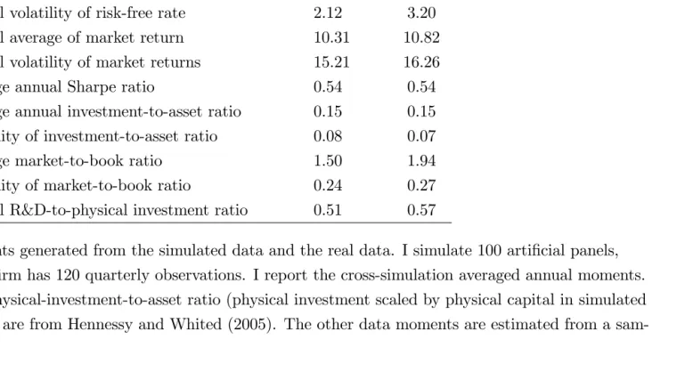
= 0:995; 0 = 23;and 1 = 900; which generate an average annual real interest rate of 1.65%, an annual volatility of real interest rate of 3.2%, an average annual stock market return of 10.82%
and an annual volatility of the stock market return of 16.26%. Those values are close to the values
obtained in the data. The calibrated Sharpe ratio of the model is 0.56, close to 0.54 for the last
30 years (1975-2005) of data.
Prior studies provide only limited guidance for the calibration of the second group of
parame-ters. These parameters are: (i)a;the weight on physical investment in im
t ;(1 )kut+1 ;(ii)11 ;
the elasticity of substitution between physical investment and intangible capital in im
t ;(1 )kut+1 ;
and (iii) A, the constant term in im
t ;(1 )kut+1 :I pin down these three parameters to match
three moments: the average annual rate of physical investment, the average annual
market-to-book ratio, and the average annual R&D investment to physical investment ratio. This procedure
yieldsa= 0:79; A= 0:42;and = 0:25. The calibrated mean and volatility of physical investment
rate in the model are 0.15 and 0.07, respectively, close to 0.15 and 0.06 reported in Hennessy and
Whited (2005). The calibrated mean and volatility of market-to-book ratio are 1.94 and 0.27,
respectively, close to 1.50 and 0.24 reported by Hennessy and Whited. The average ratio of R&D
investment to physical investment is 0.57 in the model, close to the value of 0.51 in the data. In
23Persistence
z and conditional volatility z are set to match monthly values from Zhang (2005), z= 0:973=
0:91; z= 0:10
p
sum, the calibrated parameter values seem reasonable representative of reality.
4.2
Properties of Model Solutions
In this section, I investigate the qualitative properties of the key variables in the model.
4.2.1 Marginal Cost of Investments
The formulation of the production function and the evolution of new physical capital have the
following implications for the behavior of the marginal cost of physical investment and the e¤ective
marginal cost of R&D investment:
Marginal Cost of Physical Investment
The critical variable in the model isqm
t , the equilibrium marginal cost of physical investment.
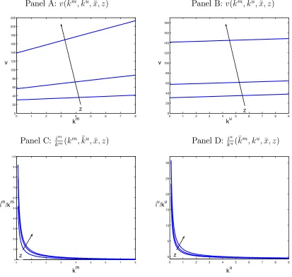
Panels A and B in Figure 1 plot the numerical examples ofqm
t as functions of physical investment
im
t and intangible capitalkut+1. In Panel A, I plotqmt against physical investmentimt in four curves,
each of which corresponds to one value of intangible capital ku
t+1; where the arrow indicates the
direction along which ku
t+1 increases. In Panel B I plot qtm against intangible capital ktu+1 in four
curves, each of which corresponds to one value of physical investmentim
t ;where the arrow indicates
the direction along which im
t increases. Marginal cost of physical investment qtm is increasing in
physical investment im
t due to diminishing-marginal-returns of imt ;(1 )kut+1 in imt ,24 and
is decreasing in intangible capital ku
t+1 because current technological progress makes new capital
production more e¢cient and less expensive.25
E¤ective Marginal Cost of R&D Investment
Panels C and D in Figure 1 plot the numerical examples of the e¤ective marginal cost of R&D
investment q~u
t as functions of physical investment imt and intangible capital ktu+1. In Panel C I
plot q~u
t against physical investment imt in four curves, each of which corresponds to one value
of intangible capital ku
t+1; where the arrow indicates the direction along which ktu+1 increases.
In Panel D I plot q~u
t against intangible capital kut+1 in four curves, each of which corresponds
24In the model,qm
t = 1
1[imt ;(1 )kut+1]
: Since 11 imt ;(1 )kut+1 <0;
@qm t @im
t >0:
25To see why this is the case, qm
t = 1
1[imt ;(1 )kut+1]
:Since 12 imt ;(1 )ktu+1 >0;
@qm t @ku
to one value of physical investment im
t ; where the arrow indicates the direction along which imt
increases. The e¤ective marginal cost of R&D investment q~u
t is decreasing in physical investment
because the term of indirect bene…t qm
t u imt ;(1 )kut+1 is increasing in physical investment.
The e¤ective marginal cost of R&D investmentq~u
t is increasing in R&D capital due to the concavity
of im
t ;(1 )kut+1 in ktu+1:
4.2.2 Value Functions and Policy Functions
Using the numerical solution to the benchmark model, I plot and discuss the value and policy
functions as functions of the underlying state variables.
Because there are four state variables (physical capital stock km
t , intangible capital stock ktu;
the aggregate productivity shock xt, and idiosyncratic productivity shock zt), and the focus of
the paper is the cross-sectional variations, I …x the aggregate productivity shock at its long-run
average, xt = x: Panels A and C in Figure 2 plot the variables against kmt and zt; with kut and
xt …xed at their long-run average levels ku and x. Panels B and D in Figure 2 plot the variables
against ku
t and zt; with kmt and xt …xed at their long-run average level km and x: Each one of
these panels has a set of curves corresponding to di¤erent values ofzt;and the arrow in each panel
indicates the direction along which zt increases.
In Panels A and B in Figure 2, the …rms’cum-dividend market value of equity is increasing in
the …rm-speci…c productivity, the physical capital stock and the intangible capital stock. Because
of constant returns to scale in the output production technology, …rm value is linear in the physical
capital stock and intangible capital stock. In Panels C and D in Figure 2, the optimal physical
investment and R&D investment are increasing in the …rm-speci…c productivity. This indicates
that the more pro…table …rms with higher …rm-speci…c productivity invest more than less pro…table
…rms with lower …rm-speci…c productivity. This …nding is consistent with the evidence documented
by Fama and French (1995). In Panels C and D of Figure 2, the optimal investment rates are
decreasing in capital stocks. Small …rms with less capital invest more and grow faster than big
…rms with more capital. That prediction is consistent with the evidence provided by Evans (1987)
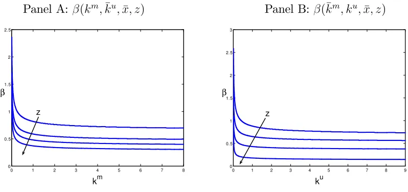
4.2.3 Fundamental Determinants of Risk
I …nd that risk, measured as t from equation (35), is decreasing in the three …rm-speci…c state variables: the physical capital stock, the intangible capital stock and the …rm-speci…c productivity.
Using the benchmark parametrization, Panels A and B of Figure 3 plot tagainst physical capital,
km
t ; and intangible capital, kut; and …rm-speci…c productivity, zt, with the aggregate productivity
…xed at its long-run averages, xt=x:Doing so allows me to focus on the cross-sectional variation
of risk. Panels A and B plot t in four curves, each of which corresponds to one value of
…rm-speci…c productivity,zt. The arrow in the panels indicates the direction along whichztincreases.
Small …rms with less physical capital are more risky than big …rms with more capital. That is
consistent with Li, Livdan and Zhang (2008). Consistent with Zhang (2005), less pro…table …rms
are riskier than more pro…table …rms, .
4.3
Empirical Predictions
Here, the quantitative implications concerning the cross section of returns in the model are
inves-tigated. I show that a neoclassic model with endogenous technological progress driven by R&D
investment is capable of simultaneously generating a positive relation between R&D investment
and the subsequent average of stock returns and a negative relation between physical investment
and the subsequent average of stock returns. The model also generates a positive relation between
book-to-market ratio and the subsequent average of stock returns.
The design of the quantitative experiment follows Kydland and Prescott (1982), Berk, Green
and Naik (1999) and Zhang (2005). I simulate 100 samples, each with 3000 …rms. And each …rm
has 120 quarterly observations. The empirical procedure on each arti…cial sample is implemented
and the cross-simulation results are reported. I then compare model moments with where possible
those in the data.
4.3.1 R&D Investment and Stock Returns
I now investigate the empirical predictions of the model on the cross section of stock returns
(2006). They document a positive relation between R&D intensity26 and the subsequent average
of stock returns. Chan, Lakonishok and Sougiannis (2001) interpret their results as indicating that
investors are overly pessimistic about R&D …rms’ prospects. Li (2006) attributes her results to the
fact that R&D …rms are more likely to be …nancially constrained. I show that a neoclassical model
without investor irrationality or …nancing frictions can quantitatively replicate their evidence.
I follow Chan, Lakonishok and Sougiannis (2001) in constructing 5 equal-weighted R&D
port-folios for each simulated panel (See Appendix C.2 for details about the empirical procedure.). The
market value of equity in the model is de…ned as the ex-dividend stock price. I sort all …rms into
5 portfolios based on …rms’ ratio of R&D investment to market value of equity, iu
t 1=pst 1;and the
ratio of R&D investment to physical investment, iu
t 1=imt 1;in ascending order as of the beginning
of year t. I then calculate the equal-weighted annual average stock returns and average excess
returns for each R&D investment portfolio. Following Chan, Lakonishok and Sougiannis (2001),
I measure excess returns relative to benchmarks constructed to have similar …rm characteristics
such as size and book-to-market (See Appendix C.1 for details about the empirical procedure.). I
construct a R&D investment-spread portfolio long in the high R&D intensity iu
t 1=pst 1; iut 1=imt 1
portfolio and short in the low R&D intensity iu
t 1=pst 1; iut 1=imt 1 portfolio. I repeat the entire
simulation 100 times and report the cross-simulation averages of the summary statistics in Table
3.
From Panel A and Panel B in Table 3, consistent with Chan, Lakonishok and Sougiannis
(2001) and Li (2006), …rms with high R&D intensity, iu
t 1=pst 1 (iut 1=imt 1), earn higher average
stock returns and higher excess returns than …rms with low R&D intensity. The model generates
a reliable R&D investment-spread in Panel B, which is 8.75% (10.03%) per annum for portfolios
sorted on iu
t 1=pst 1 and iut 1=imt 1; respectively, close to those in the data, 12.06% (11.67%).
4.3.2 Physical Investment and Stock Returns
I now investigate the empirical predictions of the model for the cross section of stock returns and
physical investment. I focus on Xing (2006), who documents that physical investment contains
26Chan, Lakonishok and Sougiannis (2001) and Li (2006) use R&D investment scaled by market value of equity,
information similar to the book-to-market ratio in explaining the value e¤ect and that …rms with
higher rate of physical investment earn lower average subsequent stock returns.
I follow Xing (2006) in constructing 10 (both value-weighted and equal-weighted) portfolios
sorted on physical investment. I sort all …rms into 10 portfolios based on …rms’ rate of physical
investment, im
t 1=kmt 1; in ascending order as of the beginning of year t. I construct a
physical-investment-spread portfolio long in the low im
t 1=ktm1 portfolio and short in the high imt 1=ktm1
portfolio, for each simulated panel. Table 4 reports the average stock returns of 10 portfolios sorted
on physical investment. Consistent with Xing (2006), …rms with low im
t 1=kmt 1 on average earn
higher stock returns than …rms with high im
t 1=kmt 1. The model-implied average value-weighted
(equal-weighted) physical investment-spread is 14.21% (17.51%) per annum. This spread is higher
than that in the data, 5.28% (5.64%).
4.3.3 Abnormal Physical Investment and Stock Returns
I now investigate the empirical predictions of the model for the cross section of stock returns
and abnormal physical investment. I focus on Titman, Wei and Xie (2004), who document that
…rms with higher abnormal physical investment, de…ned as CIm t 1 =
CEm t 1 (CEm
t 2+CEtm3+CEmt 4)=3 1 in
the portfolio formation year t; earn lower subsequent average stock returns after controlling size,
book-to-market and momentum (prior year return), where CEm
t 1 is physical capital expenditure
scaled by sales during yeart 1. Titman, Wei and Xie (2004) attribute their …ndings to investors’
underreacting to the overinvestment behavior of empire building managers. I show that a
neoclas-sical model without investor irrationality can quantitatively replicate their evidence. It is worth
noting that Li, Livdan and Zhang (2008) also generate similar quantitative results, but with a
di¤erent model.
I measure CEtm1 in the model as the physical investment-to-output ratio, imt 1=yt 1. The last
three-year moving-average physical capital expenditure in the denominator of CIm
t 1 is used to
proxy for …rms’ benchmark physical investment. I sort all …rms into quintiles based on CIm t 1 in
ascending order as of the beginning of year t. I construct a CI-spread portfolio long in the low
I calculate the value-weighted annual excess returns for eachCI portfolio. Following Titman,
Wei, and Xie (2004), I measure excess returns relative to benchmarks constructed to have similar
…rm characteristics such as size, book-to-market, and momentum. (See Appendix C.3 for details
about the empirical procedure.) Table 6 reports the average excess stock returns of 5 portfolios
sorted on abnormal physical investment,CI. Consistent with the …ndings of Titman, Wei and Xie
(2004), …rms with low CI earn higher average excess stock returns than …rms with highCI. The
model-implied average CI-spread is 2.14% per annum. This spread is close to that documented
in the data, 2.03%.
In sum, the benchmark model can simultaneously generate a positive covariation between
R&D investment and future average stock returns, and a negative covariation between physical
investment and future average stock returns.
Notably, the stochastic discount factor with countercyclical market price of risk is necessary
to generate spreads of R&D investment portfolios and physical investment portfolios that are
consistent with the data. With a constant price of risk, i.e., 1 = 0, the spreads of portfolio returns are smaller than those with a countercyclical price of risk. The results with constant price
of risk are available upon request.
4.3.4 The Value Premium
Here, I explore the relation between endogenous technological progress and the value premium.
First I investigate if the model can generate a positive relation between the book-to-market
ratio and expected stock returns. I construct 10 value-weighted and equal-weighted
book-to-market portfolios. The book value of a …rm in the model is identi…ed as its physical capital stock.
I sort all …rms into 10 portfolios based on …rms’ book-to-market ratio, km
t 1=pst 1; in ascending
order as of the beginning of year t. I construct a value-spread portfolio long in the high
book-to-market portfolio and short in the low book-to-book-to-market portfolio for each simulated panel. Table 7
reports the average stock returns of 10 portfolios sorted by book-to-market ratio. Consistent with
the …ndings of Fama-French (1992, 1993), …rms with low book-to-market ratios earn lower stock
value-weighted (equal-weighted) value-spread is 13.45% (19.27%) per annum. This spread is close
to that documented in the data, 8.72% (19.36%).
4.4
Causality
I now focus on causal relations why R&D investment positively forecasts average stock returns
while physical investment negatively forecasts average stock returns in the model. I also investigate
the relation between endogenous technological progress and the value premium.
4.4.1 Investment Returns and Investment
First I examine the covariations between investment returns (both R&D and physical) and
invest-ment. In Panel A of Table 8, I report simulated average physical investment returns and R&D
investment returns of 5 portfolios sorted on R&D intensity and rate of physical investment. The
expected return on physical investment is negatively related to physical investment but positively
related to R&D investment. This is because R&D investment increases the marginal product of
physical capital; and R&D (physical) investment decreases (increases) the marginal cost of
phys-ical investment, which is negatively related to the expected physphys-ical investment returns. The
expected returns on R&D investment covaries positively with physical investment and covaries
negatively with R&D investment. That is because the expected marginal product of R&D capital
(the e¤ective marginal cost of R&D investment) is decreasing (increasing) in R&D investment but
increasing (decreasing) in physical investment. So investments (both R&D and physical) covary
with the expected physical investment return and R&D investment return in opposite ways. That
leads to two countervailing e¤ects on the predictability of investments on future average stock
returns. We need to examine the weights on R&D investment return and physical investment
return to determine which e¤ect dominates.
4.4.2 Weights on Investment Returns
Panel B in Table 8 reports simulated average weights on physical investment return and on R&D
weight on physical investment return qmt kt+1m
ps
t is much greater than the weight on R&D investment
return q~tukut+1
ps
t . This is because physical capital production involves both intangible capital and
physical investment, and the share of intangible capital in the output production is smaller than
that of the tangible capital. The di¤erence in weights between physical investment return and
R&D investment return implies that physical investment return together with its weight qmt kt+1m
ps t r
m t+1
dominates in stock returns. That is why R&D investment positively forecasts average future stock
returns while physical investment negatively forecasts average future stock returns.
4.4.3 Endogenous Technological Progress and the Value Premium
In the model, value …rms invest less in intangible capital than do growth …rms, so value …rms do
not gain as much from technological progress in increasing the productivity of physical capital as
growth …rms do. When a recession comes, value …rms are stuck with excessive physical capital and
do not have much endogenous technological progress to upgrade the e¢ciency of physical capital.
They are therefore more risky than growth …rms, given that the price of risk is high in economic
downturns. This interaction between endogenous technological progress and physical capital
re-inforces the mechanism emphasized in Zhang (2005) who demonstrates that costly reversibility of
physical capital is one of key mechanisms driving the value premium.
4.5
Discussion
The crucial channel in the model in generating a positive relation between R&D investment and
the average stock returns is productivity increasing innovation. This is because, on one hand, if
all R&D investment is devoted to creating new products ( = 1), the model reduces to standard
models which predict that both R&D investment and physical investment forecast the expected
stock returns in the same way27, which is counterfactual; on the other hand, if all R&D investment
is dedicated to increasing productivity of physical investment ( = 0) and output production is
linear in physical capital, the model can still simultaneously explain the relationships of R&D
27Then output production has to be decreasing returns to scale in physical capital and R&D capital to guarantee
investment and physical investment with the average stock returns28.
5
Concluding Remarks
Following Cochrane (1991, 1996), I show that a neoclassical model with endogenous technological
progress driven by R&D investment can explain a number of empirical regularities in the cross
section of stock returns. Most notably, technological progress endogenously driven by R&D
invest-ment raises expected marginal bene…t of physical capital and reduces the marginal cost of physical
investment, causing expected returns in physical investment increasing in R&D investment. The
expected physical investment return is decreasing in physical investment due to diminishing
mar-ginal returns of physical capital production. In the model the weight on physical investment
return dominates the weight on R&D investment return, thus the model simultaneously explains
why R&D intensive …rms earn high average stock returns while physical
investment-intensive …rms earn low average stock returns. The positive predictability of R&D investment on
expected stock returns, interpreted by Chan et al (2001) as excessive pessimism, is in principle
consistent with rational expectations. The model also explains why value …rms are more risky than
growth …rms; value …rms invest less in R&D capital, and thus do not have as much technological
progress in upgrading the e¢ciency of the existing physical capital as growth …rms, especially in
bad times.
Future research can proceed in a few directions. Theoretically, a full-‡edged general
equilib-rium model with Epstein-Zin preferences can link endogenous technological progress to long-run
consumption risk. The neoclassical framework in the model can also be extended to link asset
prices to other types of intangible capital, e.g., human capital and organizational capital.
Em-pirically, the correlation between human capital, organizational capital and physical capital, and
their relations with the cross section of stock returns is worth further investigating.