New Implementation of Reproducing Kernel Method for Solving Functional Differential Equations

(1)

http://dx.doi.org/10.4236/am.2016.710095

How to cite this paper: Abdollazadeh, A., Moradi, F. and Pourbashash, H. (2016) New Implementation of Reproducing Ker-nel Method for Solving Functional-Differential Equations. Applied Mathematics, 7, 1074-1081.

http://dx.doi.org/10.4236/am.2016.710095

New Implementation of Reproducing Kernel

Method for Solving Functional-Differential

Equations

Aboalfazl Abdollazadeh

1

, Farhad Moradi

2

, Hossein Pourbashash

3*

1_{Department of Mathematics, Faculty of Mathematical Sciences and Statistics, Birjand University, Birjand, Iran} 2_{Department of Mathematics, Faculty of Mathematical Sciences and Computer, Kharazmi University, Tehran,} Iran

3_{Department of Mathematics, University of Garmsar, Garmsar, Iran}

Received 10 April 2016; accepted 19 June 2016; published 22 June 2016

This work is licensed under the Creative Commons Attribution International License (CC BY). http://creativecommons.org/licenses/by/4.0/

Abstract

In this paper, we apply the new algorithm of reproducing kernel method to give the approximate solution to some functional-differential equations. The numerical results demonstrate the accu-racy of the proposed algorithm.

Keywords

Reproducing Kernel Hilbert Spaces, Functional-Differential Equations, Approximate Solutions

1. Introduction

The subject of differential equations is a wide field in pure and applied mathematics, engineering, physics, chemistry, biology, psychology and other fields. All of these disciplines are associated with the properties of differential equations of various types. Pure mathematics discusses existence and uniqueness of solutions, while applied mathematics emphasizes the rigorous justification of the methods for approximating solutions. Differen- tial equations have a prominent role in modelling virtually each physical, technical and/or biological processes, from celestial motion, to bridge design, to interactions between neurons.

This paper investigates the approximate solution of the following linear functional-differential equation using new implementation of the reproducing kernel method (RKM):

( )

(

, , ,

)

,

( )

0

( )

1 0,

( )

0

( )

1 0, 0 1.

y′′ x =g x y y y′ ′′ Ay +By = Cy′ +Dy′ = < <x (1)

(2)

where g is a function of its variables, A, B, C, D are real constants and unknown function y x

( )

is continuous on the interval [0, 1]. These problems arise in many areas of applied mathematics, physics and engineering, such as fluid mechanics, gas dynamics, reaction diffusion process, nuclear physics, chemical reactor theory, geo- physics, studies of atomic structures and etc. Several numerical techniques such as finite difference approximation [1], cubic splines [2] [3], B-splines [4], Adomian decomposition method [5], differential transformation method [6] and others [7] [8] have been proposed to obtain approximate solution of these problems by some authors. The application of RKM in linear and nonlinear problems has been developed by many researchers [9]-[12]. The RKM has been treated singular linear two-point boundary value problem, singular nonlinear two- point periodic boundary value problem, nonlinear system of boundary value problem, singular integral equations, nonlinear partial differential equations and etc. in recent years in [13]-[17].

As we know, Gram-Schmidt orthogonalization process is numerically unstable, in addition it may take a lot of time to produce numerical approximation. Here, instead of using orthogonal process, we successfully make use of the basic functions which are obtained by RKM.

This paper is organized as follows. In the next section, two reproducing kernel Hilbert space (RKHS) are in-troduced. Section 3 is devoted to solve Equation (1) by new implementation of RKM. Some numerical examples are presented in Section 4. Last section is a brief conclusion.

2. Reproducing Kernel Spaces

In this section, we follow the recent work of [18] [19] and present some useful materials.

Definition 1. For a nonempty set , let

(

, .,._

)

be a Hilbert space of real-valued functions on some set

. A function k: × → is said to be the reproducing kernel of  if and only if 1. k x

( )

,. ∈, ∀ ∈x ,

2. u k x,

( )

,. _ =u x

( )

, ∀ ∈u , ∀ ∈x , (reproducing property). Also, a Hilbert space of functions

(

, .,.

)



 that possesses a reproducing kernel k is a RKHS and we denote it by

(

, .,. ,k

)



 . In the following we often denote by kx the function k x

( )

,. :tk x t

( )

, . Definition 2. W₂3

[ ]

0,1 =

{

y y′′ is an absolute continuous real-valued function on the interval

[ ]

_{0,1 ,}_y′′′_∈_L2

[ ]

_{0,1 , 0}_Ay

( )

₊_By

( )

₁ ₌_{0, 0}_Cy′

( )

₊_Dy′

( )

₁ ₌₀

}

_{. The inner product and the norm in the function}

space W₂3

[ ]

0,1 are defined as follows:

( ) ( )

3 3 3

2 2 2

1

0

, _W 0 0 0 0 d , ,_W _W .

y v =y′ v′ +y′′ v′′ +

∫

y′′′ x v′′′ x x y = y y

Suppose that function Rx∈W23

[ ]

0,1 satisfies the following generalized differential equations

( )

(

)

( )

6 3

6

4 2 3 4 3

1 ,

0 0 0 0 1 1

0, 0, 0, 0.

x

x x x x x x

R t

t x t

R R R R R R

t t t t t t

δ

 ∂

− = −



 ∂



∂ ∂ ∂ ∂ ∂ ∂

 ₊ ₌ ₋ ₌ ₌ ₌

 ∂ ∂ ∂ ∂ ∂ ∂



(2)

where δ is the Dirac delta function, therefore the following theorem holds.

Theorem 1 Under the assumptions of Equation (2), Hilbert space W₂3

[ ]

0,1 is a RKHS with the reproducing kernel function Rx, namely for any

[ ]

3 2 0,1

y W∈ and each fixed x∈

[ ]

0,1 ,

( )

3 2

, _{x W} .

y R =y x

Proof. Applying integration by parts three times, since R_x∈W₂3

[ ]

0,1 , we have

( )

3 2

2 3

1

2 0 3

4 2 3

3 4 6

1

3 4 0 6

0 0

, 0 0 d

0 0 0 0

0 0

1 1

1 1 d .

x x x

x W

x x x x

x x x

R R R t

y R y y y t t

t t t

R R R R

y y

t t t t

R R R t

y y y t t

t t t

∂ ∂ ∂

′ ′′ ′′′

= + +

∂ ∂ ∂

∂ ∂  ∂ ∂ 

′ ′′

=  + +  − 

∂ ∂ ∂ ∂

   

   

∂ ∂ ∂

′′ ′

+ − −

∂ ∂ ∂

∫

(3)

Therefore, Equation (2) implies that

( ) (

)

( )

3 2 1 0

, _{x W} d .

y R =

∫

y t δ t−x t=y x



While x≠t, function R_x

( )

t is the solution of the following constant linear homogeneous differential equation with 6 order,

( )

6 6 0, x R t t ∂ =

∂ (3) with the boundary condition:

( )

4 3

2 3 4

0 0 1

0, 0,

0 0 1

0, 0.

x x x

R R R

t t t

R R R

t t t

 ∂ ∂ ∂ + = =   ∂ ∂ ∂  ∂ ∂ ∂  ₋ ₌ ₌  ∂ ∂ ∂  (4)

We know that Equation (3) has characteristic equation λ =6 0, and the eigenvalue λ=0 is a root whose multiplicity is 6. Hence, the general solution of Equation (2) is

( )

6 1 1 6 1 1 , , , . i i i x i i i

c x t t x

R t

d x t t x

− = − =  _≤  =   _> 

∑

(5)

Now, we are ready to calculate the coefficients c x_i

( )

and di

( )

x , 1,i= , 6. Since

( )

₍

₎

6 6 , x R t t x t δ ∂ = − ∂ we have

( )

5 5 5 5

, 0, , 4,

1.

k k

x x

k k

x x

R x R x

k

t t

R x R x

t t + − + − ∂ ∂  = =  ∂ ∂  ∂ ∂  − = −  ∂ ∂   (6)

Then, using Equations (4) and (6), the unknown coefficients of Equation (5) are uniquely obtained. Therefore,

( )

(

2

₍

)

₎

5 3

(

_{( )}

)

42

₎

(

₍

)

₎

3 24

₍

( )

2

₎

25

1 120 1 24 1 12 1 4 , ,

1 12 1 4 1 24 1 120 , ,

x

t t x t x t x t x

R t

t x x tx x t x

 − + + ≤

 = 

+ − + >



Definition 3. 1

[ ]

2 0,1

W = {y y is an absolute continuous real-valued function on the interval

[ ]

0,1 ,

[ ]

2 0,1

y′∈L }. The inner product and the norm in the function space W₂1

[ ]

0,1 are defined as follows:

( ) ( )

1 1 1

2 2 2

1

0

, 0 0 d , .

W W W

y v =y v +

∫

y x v x′ ′ x y， = y y

Theorem 2 Hilbert space W₂1

[ ]

0,1 is a reproducing kernel space with the reproducing kernel function

( )

1 , ,

1 , .

x

t t x

r t

x t x

+ ≤



=  ₊ _> 

Theorem 3 (see [20]) Let

{ }

=1 i i

x ∞ be a dense subset of interval

[ ]

0,1 then

{

( )

}

=1

i

x i

r x ∞ is a basis of

[ ]

1 2 0,1

W .

3. The New Implementation of the Method

(4)

[ ]

3 2 0,1

W . We suppose that Equation (1) has a unique solution. We consider Equation (1) as

( )

x = f x y y y

(

, , ′ ′′,

)

, 0≤ ≤x 1,

 (7)

where y x

( )

= p x y

( ) ( )

′′ x and f x y y y

(

, , ′ ′′,

)

= p x g x y y y

( ) (

, , ′ ′′,

)

, such that f is an analytical function. It is clear that  is the bounded linear operator of W23

[ ]

0,1 into

[ ]

1 2 0,1

W . We shall give the representation of

analytical solution of Equation (7) in the space W₂3

[ ]

0,1 . Put

( )

i

i x rx x

ϕ

= and

ψ

_i

( )

x =*

ϕ

_i

( )

x i, =1, 2,, where

( )

i

x

r x is the reproducing kernel of W21

[ ]

0,1 and

∗

 is the adjoint operator of .

Theorem 4 Let

{ }

1 i i

x ∞₌ be a dense subset of interval

[ ]

0,1 , then

{

( )

}

1

i x _i

ψ ∞₌ is a complete system of

[ ]

3 2 0,1

W and

( )

i

i x tR tx _x

ψ

=_ , where the subscript t in the operator  indicates that the operator  applies to the function of t.

Proof. For each fixed y W∈ 23

[ ]

0,1 , let 3 2

, _{i W} 0, 1, 2, ,

yψ = i=  which means that

( )

1

3 ₂

2

*

, i , i _W i 0, 1, 2, .

W

y 

ϕ

= y

ϕ

=y x = i= 

Note that

{ }

1 i i

x ∞₌ is dense on

[ ]

0,1 , hence, y x

( )

=0. Due to the existence of −1, then y≡0. There- fore,

{

( )

}

1

i x _i

ψ ∞₌ is the complete system of W₂3

[ ]

0,1 . Now, note that

( )

1 3 ₂ 2 1 2 * * , , , | . i i

i i i x i _{x W}

W

x x t x t x

W

x x R R

R R R t

ψ ϕ ϕ ϕ

= = = = = =     



Usually, a normalized orthogonal system is constructed from

{

( )

}

1

i x _i

ψ ∞

= by using the Gram-Schmidt

algorithm, and then the approximate solution will be obtained by calculating a truncated series based on these functions. However, Gram-Schmidt algorithm has some drawbacks such as numerical instability and high volume of computations. Here, to fix these flaws, we state the following Theorem in which the following notations are used.

1

1 11

1

2 21 22

2 2

1 2

ˆ

ˆ 0 0

ˆ

ˆ 0

ˆ , , , ,

ˆN N ˆ N N NN

N f a a a a f B a a _f β β β

β β β

  _…     _ _       _ _  _…        = = =_ _ =     _ _       _ _   …       _ _

a a F

    

 

where ˆf_i = f,ψ_i , 0, 1,β_ii > i= ,N. And

11 12 1 11 12 1

21 22 2 21 22 2

1 2 1 2

, ,

N N

N N NN N N NN

ψ ψ ψ ψ ψ ψ

… …

   

 _…   _… 

   

Ψ = Ψ =

        … …                      

where ψ_ij = ψ ψ ψ_j, _i , _ij = ψ ψ _j, _i , ,i j=1,,N.

Theorem 5 Suppose that

{

( )

}

1

i x _i

ψ ∞

= is a linearly independent set in

[ ]

3 2 0,1

W and

{

( )

}

1

i x _i

ψ ∞

=

 be a norma-

lized orthogonal system in W₂3

[ ]

0,1 , such that

( )

1

i

i x k ik k x ψ =

∑

₌β ψ . If

( )

1

( )

1

( )

1ˆ

( )

N N

i i N i i i i

i i i

y x =

∑

∞₌ aψ x y x =

∑

₌ aψ x =

∑

₌aψ x then Ψ =a F. Proof. Suppose that y W∈ ₂3

[ ]

0,1 then

( )

1 i i 1ˆi i .

i i

y x =

∑

∞₌ aψ x =

∑

∞₌ aψ x Now, by truncating N-term of

the two series, because of

( )

1 1ˆ

N i i i i i i

y x =

∑

∞₌ aψ x =

∑

∞₌ aψ x and since

( )

1

i

(5)

( )

1 1 1 1 1

ˆ ˆ ˆ .

N N N i N N

i i i i i ik k i ik k

i i i k k i k

aψ x aψ x a β ψ x aβ ψ x

= = = = = =

 

= = = _ _

 

∑



∑ ∑

Due to the linear independence of

{

( )

}

1

i x _i

ψ ∞₌ , _k N ˆ_i _ik, 1, , i k

a =

∑

₌ aβ k=  N therefore T_ˆ.

B

=

a a (8)

Equation (7), imply y_N

( )

x = f x

( )

. For i=1,,N we have

(

)

(

)

1

1 1 1 1

T

1 1 1 1

T

1 1

T

ˆ

, , , ,

ˆ , ,

ˆ .

N

N i i j j i i

j

N i i

j ik jl l k ik k

j k l k

j

N i i

j ik l k lj ik k

j k l k

N i

j ik k

ij

j k

y f a f

a f

a B B f

B B B

ψ ψ ψ ψ ψ

β β ψ ψ β ψ

β ψ ψ β β ψ

β ψ

=

= = = =

= =

= ⇒ =

⇒ =

⇒ Ψ =

∑

∑ ∑ ∑

∑

∑ ∑∑

∑

a F

    

 



Equation (8), imply BΨ =a BF, hence

.

Ψ =a F



It is necessary to mention that here we solve the system Ψ =a F. which obtained without using the Gram- Schmidt algorithm.

4. Numerical Examples

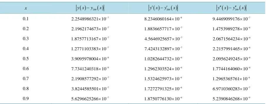
To illustrate the effectiveness of the proposed method, some numerical examples are considered in this section. The numerical results in Table 1 and Table 2 show that the approximate solution and its derivatives up to second order, converge to the exact solution and its derivatives respectively. The examples are computed by using Maple 18.

Example 1. Consider the following second-order ordinary differential equation with singular coefficients

( )

3 1

1 1 1 , 0 1,

2 2 2

0 0, 0 0,

x x

y x y x x g x x

x

y y

 ₋  _′′ ₊  ₋  _′ ₊ ₋  ₌ _{< <}

     

     

′

= =

[image:5.595.88.540.545.722.2]

(9)

Table 1. Absolute errors for Example 1 with CPU time 46.582 in seconds.

x y x( )−y200( )x y x′( )−y200′ ( )x y′′( )x −y200′′ ( )x

0.1 7

2.2548986321 10× − 8

8.2346060164 10× − 7

9.4469099176 10× −

0.2 7

2.1962174673 10× − 7

1.8836657717 10× − 6

1.4753989278 10× −

0.3 7

1.8757713167 10× − 7

4.5646925657 10× − 6

2.0671564234 10× −

0.4 7

1.2771103383 10× − 7

7.4243132897 10× − 6

2.2157991465 10× −

0.5 8

3.9095978004 10× − 6

1.0282644732 10× − 6

2.0956249245 10× −

0.6 8

7.7341240318 10× − 6

1.2962303524 10× − 6

1.7744164060 10× −

0.7 7

2.1908577292 10× − 6

1.5324625973 10× − 6

1.2965365761 10× −

0.8 7

3.8244585501 10× − 6

1.7272791325 10× − 7

6.9710360283 10× −

0.9 7

5.6296625266 10× − 6

1.8750776130 10× − 9

(6)

where

( )

2 3 4

29 13 3

5

2 2 2 2

x x x x

g x = − + + − . The exact solution is y x

( )

=x2−x3.

Example 2. We consider the following second-order delay differential equation

( )

1

3, 0 1,

2 2 2

0 1, 0 0,

x x

y x y y x x

y y

   

′′ = ′_{ }− ′′_{ }− + < <

   

′

= =

(10)

with exact solution y x

( )

= +1 x2.

Remark 1. The RKM is tested on these problems with gird points x_i i , 1,i ,N

N

= =  for N=20, 200. The

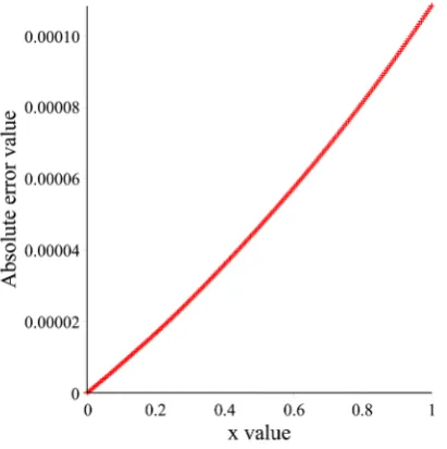
[image:6.595.86.539.277.480.2]

numerical results for Example 1 and 2 are listed in Table 1, Table 2 and Figure 1, Figure 2. The results shown in Table 1, Table 2, indicate that the approximate solution and its derivatives up to second order, converge to the exact solution and its derivatives respectively.

Table 2. Absolute errors for Example 2 with CPU time 14.321 in seconds.

x y x( )−y200( )x y x′( )−y200′ ( )x y′′( )x −y200′′ ( )x

0.1 8

5.2264693462 10× − 6

1.0611304470 10× − 6

3.3094355000 10× −

0.2 7

1.0436888331 10× − 8

6.4357294000 10× − 7

5.0328956000 10× −

0.3 7

1.3870091453 10× − 7

7.4194858790 10× − 6

7.9044009800 10× −

0.4 7

2.4136835086 10× − 6

1.1820612788 10× − 7

3.9655752000 10× −

0.5 7

3.5146566701 10× − 7

9.5106389175 10× − 6

3.7509744025 10× −

0.6 7

4.2789167831 10× − 7

5.8832386536 10× − 6

3.1381459680 10× −

0.7 7

4.7405615700 10× − 7

3.6855082200 10× − 6

1.1318180400 10× −

0.8 7

5.0902815873 10× − 7

3.6716689840 10× − 6

1.0503155200 10× −

0.9 7

5.5388322306 10× − 7

5.5412781980 10× − 6

2.5048595280 10× −

(7)

[image:7.595.214.420.87.294.2]

Figure 2. The absolute error between exact and approximate solutions for Example 2 with N = 20.

5. Conclusion

In this paper, it is shown that the RKM without Gram-Schmidt algorithm is quiet efficient and well suited for finding the approximate solutions to some two-order initial value problems. We obtained the numerical solutions, with high accuracy and moderate CPU time. The numerical results obtained here, indicate the high performance of this method for approximating solution of functional-differential equations.

Acknowledgements

We thank the Editor and the referees for their comments.

References

[1] Kanth, A.S.V.R. and Reddy, Y.N. (2004) Higher Order Finite Difference Method for a Class of Singular Boundary Value Problems. Applied Mathematics and Computation, 155, 249-258.

http://dx.doi.org/10.1016/S0096-3003(03)00774-4

[2] Kanth, A.S.V.R. and Reddy, Y.N. (2005) Cubic Spline for a Class of Singular Boundary Value Problems. Applied

Mathematics and Computation, 170, 733-740. http://dx.doi.org/10.1016/j.amc.2004.12.049

[3] Mohanty, R.K., Sachder, P.L. and Jha, N. (2004) An

( )

4

O h Accurate Cubic Spline TAGE Method for Nonlinear

Singular Two Point Boundary Value Problem. Applied Mathematics and Computation, 158, 853-868. http://dx.doi.org/10.1016/j.amc.2003.08.145

[4] Kadalbajoo, M.K. and Aggarwal, V.K. (2005) Numerical Solution of Singular Boundary Value Problems via Cheby-shev Polynomial and B-Spline. Applied Mathematics and Computation, 160, 851-863.

http://dx.doi.org/10.1016/j.amc.2003.12.004

[5] Ebaid, A. (2011) A New Analytical and Numerical Treatment for Singular Two-Point Boundary Value Problems via the Adomian Decomposition Method. Journal of Computational and Applied Mathematics, 235, 1914-1924.

http://dx.doi.org/10.1016/j.cam.2010.09.007

[6] Ravi Kanth, A.S.V. and Aruna, K. (2008) Solution of Singular Two-Point Boundary Value Problems Using Differen-tial Transformation Method. Physics Letters A, 372, 4671-4673. http://dx.doi.org/10.1016/j.physleta.2008.05.019

[7] Babolian, E., Bromilow, M., England, R. and Saravi, M. (2007) A Modification of Pseudo-Spectral Method for Solving a Linear ODEs with Singularity. Applied Mathematics and Computation, 188, 1260-1266.

(8)

http://dx.doi.org/10.1016/S0096-3003(01)00197-7

[9] Wang, W., Cui, M. and Han, B. (2008) A New Method for Solving a Class of Singular Two-Point Boundary Value Problems. Applied Mathematics and Computation, 206, 721-727. http://dx.doi.org/10.1016/j.amc.2008.09.019

[10] Geng, F. and Cui, M. (2008) Solving Singular Nonlinear Two-Point Boundary Value Problems in the Reproducing Kernel Space. Journal of the Korean Mathematical Society, 45, 631-644.

[11] Geng, F. and Cui, M. (2007) Solving Singular Nonlinear Second-Order Periodic Boundary Value Problems in the Re-producing Kernel Space. Applied Mathematics and Computation, 192, 389-398.

[12] Cui, M. and Geng, F. (2007) Solving Singular Two-Point Boundary Value Problem in Reproducing Kernel Space.

Journal of Computational and Applied Mathematics, 205, 6-15. http://dx.doi.org/10.1016/j.cam.2006.04.037

[13] Geng, F. (2009) Solving Singular Second Order Three-Point Boundary Value Problems Using Reproducing Kernel Hilbert Space Method. Applied Mathematics and Computation, 215, 2095-2102.

[14] Lin, Y., Niu, J. and Cui, M. (2012) A Numerical Solution to Nonlinear Second Order Three-Point Boundary Value Problems in the Reproducing Kernel Space. Applied Mathematics and Computation, 218, 7362-7368.

[15] Yulan, W., Chaolu, T. and Jing, P. (2009) New Algorithm for Second-Order Boundary Value Problems of Inte-gro-Differential Equation. Journal of Computational and Applied Mathematics, 229, 1-6.

[16] Geng, F. and Cui, M. (2007) Solving a Nonlinear System of Second Order Boundary Value Problems. Journal of

Ma-thematical Analysis and Applications, 327, 1167-1181. http://dx.doi.org/10.1016/j.jmaa.2006.05.011

[17] Mohammadi, M. and Mokhtari, R. (2011) Solving the Generalized Regularized Long Wave Equation on the Basis of a Reproducing Kernel Space. Journal of Computational and Applied Mathematics, 235, 4003-4014.

[18] Aronszajn, N. (1950) Theory of Reproducing Kernel.Transactions of the American Mathematical Society, 68, 337-404. http://dx.doi.org/10.1090/S0002-9947-1950-0051437-7

[19] Cui, M. and Lin, Y. (2009) Nonlinear Numerical Analysis in Reproducing Kernel Hilbert Space. Nova Science Pub-lisher, New York.

[20] Chen, Z. and Zhou, Y. (2011) A New Method for Solving Hilbert Type Singular Integral Equations. Applied